Download

1 / 36
360 likes | 510 Vues
This lecture outlines the concepts of Pair-Hidden Markov Models (Pair-HMMs) and Conditional Random Fields (CRFs), two critical models in computational biology. It provides a recap of Hidden Markov Models (HMMs) and discusses their extensions to Pair-HMMs, used for tasks such as comparative gene recognition and protein secondary structure prediction. The lecture further explores how algorithms for single-sequence HMMs can be adapted for pairwise alignments. Valuable resources, including books and online materials, are recommended for deeper understanding.

E N D
Pair-HMMs and CRFs Chuong B. Do CS262, Winter 2009 Lecture #8
Outline • I’ll cover two different topics today • pair-HMMs • conditional random fields (CRFs) • Other resources • For more information on pair-HMMs, see the Durbin et al. book • For more information on CRFs, see the materials online.
Quick recap of HMMs • Formally, an HMM = (Σ, Q, A, a0, e). • alphabet: Σ = {b1, …, bM} • set of states: Q = {1, …, K} • transition probabilities: A = [aij] • initial state probabilities: a0i • emission probabilities: ei(bk) • Example: 0.05 0.95 0.95 FAIR LOADED 0.05
3 basic questions for HMMs • Evaluation: Given a sequence of observations x and a sequence of states π, compute P(x, π) • Decoding: Given a sequence of observations x, compute the maximum probability sequence of states πML = arg maxπ P(x, π) • Learning: Given an HMM with unspecified parameters θ = (A, a0, b), compute the parameters that maximize the likelihood of x and π, i.e., θML = arg maxθ P(x, π | θ)
Pair-HMMs • Roughly speaking, the generalization of HMMs with 1 observation sequence to 2 observation sequences. • Unfortunately, the usage of the term “pair-HMM” has come to mean two very different types of models in computational biology. I’ll talk about both.
Pair-HMMs: Usage #1 • Consider the HMM = (Σ1 x Σ2, Q, A, a0, e). • Alphabet consists of pairs of letters – one letter from Σ1 paired with one letter from Σ2. • Example: Dishonest casino dealer playing two games at once. 0.05 0.95 0.95 HONEST CHEAT 0.05
Pair-HMMs: Usage #1 (continued) • QUESTION: How do we handle the 3 basic questions? (evaluation, decoding, learning) • QUESTION: How would you generalize to 3 sequences? What about K sequences? Why might this be a bad idea? • Where this version of pair-HMMs comes up in practice: • Comparative gene recognition using pairwise alignments • Protein secondary structure prediction using pairwise alignments as input • etc.
Pair-HMMs: Usage #2 • Consider the HMM = ((Σ1 U {η}) x (Σ2 U {η}), Q, A, a0, e). • Similar to Usage #1, except that this time, instead of emitting a pair of letters in every state, in some states we may choose to emit a letter paired with η (the empty string). • For simplicity, we’ll assume that η is never emitted for both observation sequences simultaneously. • We’ll call the two observation sequences x and y.
Application: sequence alignment • Consider the following pair-HMM: 1 – 2 • QUESTION: What are the interpretations of P(c,d) and Q(c) for c,d Σ? • QUESTION: What does this model have to do with alignments? • QUESTION: What is the average length of a gapped region in alignments generated by this model? Average length of matched regions? M P(xi, yj) 1 – 1 – I P(xi, η) J P(η, yj) optional c Σ, P(η, c) = P(c, η) = Q(c)
Pair-HMMs: Usage #2 (continued) • Key difference from Usage #1: In these pair-HMMs, we cannotrely on the algorithms for single-sequence HMMs in order to do inference. • However, we can modify the algorithms for single sequence HMMs to work for alignment pair-HMMs.
Recap: Viterbi for single-sequence HMMs • Algorithm: • Define Vk(i) = max π1 … πi-1 P(x1 … xi-1, π1 … πi-1, xi, πi = k) • Compute using dynamic programming! 1 1 1 1 1 … 2 2 2 2 2 2 … … … … … K K K K K … x1 x2 x3 xK
(Broken) Viterbi for pair-HMMs • In the single sequence case, we defined Vk(i) = max π1 … πi-1 P(x1 … xi-1, π1 … πi-1, xi, πi = k) = ek(xi) ∙ maxjajkVj(i - 1) • QUESTION: What’s the computational complexity of DP? • Observation: In the pairwise case (x1, y1) … (xi -1, yi-1) no longer correspond to the first i– 1 letters of x and y respectively. • QUESTION: Why does this cause a problem in the pair-HMM case?
(Fixed) Viterbi for pair-HMMs • We’ll just consider this special case: • A similar trick can be used when working with the forward/backward algorithms (see Durbin et al for details) • QUESTION: What’s the computational complexity of DP? 1 – 2 • VM(i, j) = P(xi, yj) max • VI(i, j) = Q(xi) max • VJ(i, j) =Q(yj) max (1 - 2δ) VM(i - 1, j - 1) (1 - ε) VI(i - 1, j - 1) (1 - ε) VI(i - 1, j - 1) δ VM(i - 1, j) ε VI(i - 1, j) δ VM(i, j - 1) ε VJ(i, j - 1) M P(xi, yj) 1 – 1 – I P(xi, η) J P(η, yj) optional c Σ, P(η, c) = P(c, η) = Q(c)
Connection to NW with affine gaps • VM(i, j) = P(xi, yj) max • VI(i, j) = Q(xi) max • VJ(i, j) =Q(yj) max (1 - 2δ) VM(i - 1, j - 1) (1 - ε) VI(i - 1, j - 1) (1 - ε) VI(i - 1, j - 1) δ VM(i - 1, j) ε VI(i - 1, j) δ VM(i, j - 1) ε VJ(i, j - 1) • QUESTION: How would the optimal alignment change if we divided the probability for every single alignment by ∏i=1 … |x| Q(xi) ∏j = 1 … |y| Q(yj)?
Connection to NW with affine gaps VM(i, j) = P(xi, yj) max VI(i, j) = max VJ(i, j) = max (1 - 2δ) VM(i - 1, j - 1) (1 - ε) VI(i - 1, j - 1) (1 - ε) VI(i - 1, j - 1) δ VM(i - 1, j) ε VI(i - 1, j) δ VM(i, j - 1) ε VJ(i, j - 1) • Account for the extra terms “along the way.” Q(xi) Q(yj)
Connection to NW with affine gaps log VM(i, j) = P(xi, yj) + max log VI(i, j) = max log VJ(i, j) = max log (1 - 2δ) + log VM(i - 1, j - 1) log (1 - ε) + log VI(i - 1, j - 1) log (1 - ε) + log VI(i - 1, j - 1) log δ + VM(i - 1, j) log ε + VI(i - 1, j) log δ + VM(i, j - 1) log ε + VJ(i, j - 1) • Take logs, and ignore a couple terms. log Q(xi) Q(yj)
Connection to NW with affine gaps M(i, j) = S(xi, yj) + max I(i, j) = max J(i, j) = max M(i - 1, j - 1) I(i - 1, j - 1) J(i - 1, j - 1) d + M(i - 1, j) e + I(i - 1, j) d + M(i, j - 1) e + J(i, j - 1) • Rename!
Summary of pair-HMMs • We briefly discussed two types of pair-HMMs that come up in the literature. • We talked about pair-HMMs for sequence alignment. • We derived a Viterbi inference algorithm for alignment pair-HMMs and showed its rough “equivalence” to Needleman-Wunsch with affine gap penalties.
Motivation • So far, we’ve seen HMMs, a type of probabilistic model for labeling sequences. • For an input sequence x and a parse π, an HMM defines P(π, x) • In practice, when we want to perform inference, however, what we really care about is P(π | x). • In the case of the Viterbi algorithm, arg maxπ P(π | x) = arg maxπ P(x, π). • But when using posterior decoding, need P(π | x). • Why do need to parameterize P(x, π)? If we really are interested in the conditional distribution over possible parses π for a given input x, can’t we just model of P(π | x) directly? • Intuition: P(x, π) = P(x) P(π | x) why waste effort modeling P(x)?
Conditional random fields • Definition where F : state x state x observations x index Rn “local feature mapping” w Rn “parameter vector” • Summation is taken over all possible state sequences π’1 … π’|x| • aTb for two vectors a, b Rn denotes the inner product, ∑i=1 ... n ai bi exp(∑i=1 … |x| wTF(πi, πi-1, x, i)) P(π | x) = ∑π’ exp(∑i=1 … |x| wTF(π’i, π’i-1, x, i)) partition coefficient
Interpretation of weights • Define “global feature mapping” Then, • QUESTION: If all features are nonnegative, what is the effect of increasing some component wj? F(x, π) = ∑i=1 … |x| wTF(πi, πi-1, x, i) exp(wTF(x, π)) P(π | x) = ∑π’ exp(wTF(x, π’))
Relationship with HMMs • Recall that in an HMM, log P(x, π) = log P(π0) + ∑i=1 … |x| [ log P(πi | πi-1) + log P(xi | πi) ] = log a0(π0) + ∑i=1 … |x| [ log a(πi-1, πi) + log eπi(xi) ] • Suppose that we list the logarithms of all the parameters of our model in a long vector w. log a0(1) … log a0(K) log a11 … log aKK log e1(b1) … log eK(bM) w = Rn
Relationship with HMMs log P(x, π) = log a0(π0) + ∑i=1 … |x| [ log a(πi-1, πi) + log eπi(xi) ] (*) • Now, consider a feature mapping with the same dimensionality as w. For each component wj, define Fj to be a 0/1 indicator variable indicating whether the corresponding parameter should be included in scoring x, π at position i: • Then, log P(x, π) = ∑i=1 … |x| wT F(πi, πi-1, x, i). log a0(1) … log a0(K) log a11 … log aKK log e1(b1) … log eK(bM) 1{i = 1 Λπi-1 = 1} … 1{i = 1 Λπi-1 = K} 1{πi-1 = 1 Λπi = 1} … 1{πi-1 = K Λπi = K} 1{xi = b1Λπi = 1} … 1{xi = bMΛπi = K} w = F(πi, πi-1, x, i) = Rn Rn
Relationship with HMMs log P(x, π) = ∑i=1 … |x| wT F(πi, πi-1, x, i) • Equivalently, • Therefore, an HMM can be converted to an equivalent CRF. exp(∑i=1 … |x| wT F(πi, πi-1, x, i)) P(x, π) P(π | x) = = ∑π P(x, π) ∑π’ exp(∑i=1 … |x| wT F(πi, πi-1, x, i))
CRFs ≥ HMMs • All HMMs can be converted to CRFs. But, the reverse does not hold true! • Reason #1: HMM parameter vectors obey certain constraints (e.g., ∑i a0i = 1) but CRF parameter vectors (w) are unconstrained! • Reason #2: CRFs can contain features that are NOT possible to include in HMMs.
CRFS ≥ HMMs (continued) • In an HMM, our features were of the form • I.e., when scoring position i in the sequence, feature only considered the emission xi at position i. • Cannot look at other positions (e.g., xi-1, xi+1) since that would involve “emitting” a character more than once – double-counting of probability! • CRFs don’t have this problem. • Why? Because CRFs don’t attempt to model the observations x! F(πi, πi-1, x, i) = F(πi, πi-1, xi, i)
Examples of non-local features for CRFs • Casino: • Dealer looks at previous 100 positions, and determines whether at least 50 over them had 6’s. Fj(LOADED, FAIR, x, i) = 1{ xi-100 … xi has > 50 6s } • CpG islands: • Gene occurs near a CpG island. Fj(*, EXON, x, i) = 1{ xi-1000 … xi+1000 has > 1/16 CpGs }.
3 basic questions for CRFs • Evaluation: Given a sequence of observations x and a sequence of states π, compute P(π | x) • Decoding: Given a sequence of observations x, compute the maximum probability sequence of states πML = arg maxπ P(π | x) • Learning: Given a CRF with unspecified parameters w, compute the parameters that maximize the likelihood of π given x, i.e., wML = arg maxw P(π | x, w)
Viterbi for CRFs • Note that: • We can derive the following recurrence: • Notes: • Even though the features may depend on arbitrary positions in x, the sequence x is constant. The correctness of DP depends only on knowing the previous state. • Computing the partition function can be done by a similar adaptation of the forward/backward algorithms. exp(∑i=1 … |x| wTF(πi, πi-1, x, i)) argmaxπ P(π | x) = argmaxπ ∑π’ exp(∑i=1 … |x| wTF(π’i, π’i-1, x, i)) = arg maxπ exp(∑i=1 … |x| wTF(πi, πi-1, x, i)) = arg maxπ ∑i=1 … |x| wTF(πi, πi-1, x, i) • Vk(i) = maxj [ wTF(k, j, x, i) + Vj(i-1) ]
3 basic questions for CRFs • Evaluation: Given a sequence of observations x and a sequence of states π, compute P(π | x) • Decoding: Given a sequence of observations x, compute the maximum probability sequence of states πML = arg maxπ P(π | x) • Learning: Given a CRF with unspecified parameters w, compute the parameters that maximize the likelihood of π given x, i.e., wML = arg maxw P(π | x, w)
Learning CRFs • Key observation: – log P(π | x, w) is a differentiable, convex function of w convex function f(x) f(y) Any local minimum is a global minimum.
Learning CRFs (continued) • Compute partial derivative of log P(π | x, w) with respect to each parameter wj, and use the gradient ascent learning rule: Gradient points in the direction of greatest function increase w
The CRF gradient • It turns out (you’ll show this on your homework) that • This has a very nice interpretation: • We increase parameters for which the correct feature values are greater than the predicted feature values. • We decrease parameters for which the correct feature values are less than the predicted feature values • This moves probability mass from incorrect parses to correct parses. (/wj) log P(π | x, w) = Fj(x, π) – Eπ’ P(π’ | x, w) [ Fj(x, π’) ] correct value for jth feature expected value for jth feature (given the current parameters)
Summary of CRFs • We described a probabilistic model known as a CRF. • We showed how to convert any HMM into an equivalent CRF. • We mentioned briefly that inference in CRFs is very similar to inference in HMMs. • We described a gradient ascent approach to training CRFs when true parses are available.