Download
1 / 54
540 likes | 732 Vues
Light and the Electromagnetic Spectrum. Electromagnetic energy (“light”) is characterized by wavelength frequency amplitude. 1. m. m. s. s. s. Light and the Electromagnetic Spectrum. Wavelength x Frequency = Speed. . . x. =. c. m.

E N D
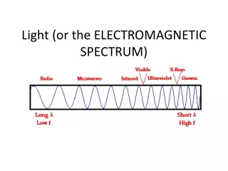
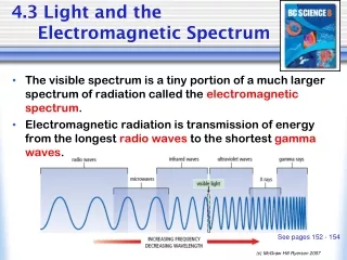
Light and the Electromagnetic Spectrum • Electromagnetic energy (“light”) is characterized by • wavelength • frequency • amplitude
1 m m s s s Light and the Electromagnetic Spectrum Wavelength x Frequency = Speed x = c m c is defined to be the rate of travel of all electromagnetic energy in a vacuum and is a constant value—speed of light. c = 3.00 x 10⁸
1 m m 1 x 10⁹ nm s c = = Light and the Electromagnetic Spectrum The light blue glow given off by mercury streetlamps has a wavelength of 436 nm. What is the frequency in hertz? Wavelength () x Frequency (f) = Speed of light x = c 3.00 x 10⁸ 436 nm = 6.88 x 10¹⁴ s-1 = 6.88 x 10¹⁴ Hz
Electromagnetic Energy and Atomic Line Spectra Excite an atom and what do you get? Light emission Line Spectrum: A series of discrete lines on an otherwise dark background as a result of light emitted by an excited atom.
= R∞ = R∞ 1 1 1 1 1 1 - - m2 22 n2 n2 Electromagnetic Energy and Atomic Line Spectra Johann Balmer in 1885 discovered a mathematical relationship for the four visible lines in the atomic line spectra for hydrogen. Johannes Rydberg later modified the equation to fit every line in the entire spectrum of hydrogen. (m & n are integers where n>m) R (Rydberg Constant) = 1.097 x 10⁻² nm-1
Particle-like Properties of Electromagnetic Energy Photoelectric Effect: Irradiation of clean metal surface with light causes electrons to be ejected from the metal. Furthermore, the frequency of the light used for the irradiation must be above some threshold value, which is different for every metal.
Particle-like Properties of Electromagnetic Energy Einstein explained the effect by assuming that a beam of light behaves as if it were a stream of particles called photons.
E Particle-like Properties of Electromagnetic Energy E = h h (Planck’s constant) = 6.626 x 10⁻³⁴ J s Electromagnetic energy (light) is quantized. Quantum: The amount of energy corresponding to one photon of light.
Particle-like Properties of Electromagnetic Energy • Niels Bohr proposed in 1914 a model of the hydrogen atom as a nucleus with an electron circling around it. • In this model, the energy levels of the orbits are • “quantized” • that is, only certain specific orbits corresponding to certain specific energies are available for the electron.
h = mv Wave-like Properties of Matter Louis de Broglie in 1924 suggested that, if light can behave in some respects like matter, then perhaps matter can behave in some respects like light. In other words, perhaps matter is wave-like as well as particle-like. The de Broglie equation allows the calculation of a “wavelength” of an electron or of any particle or object of mass m and velocity v.
Quantum Mechanics and the Heisenberg Uncertainty Principle In 1926 Erwin Schrödinger proposed the quantum mechanical model of the atom which focuses on the wavelike properties of the electron. In 1927 Werner Heisenberg stated that it is impossible to know precisely where an electron is and what path it follows—a statement called the Heisenberg uncertainty principle.
Probability of finding electron in a region of space (2) solve Wave function or orbital () Wave equation Wave Functions and Quantum Numbers A wave function is characterized by three parameters called quantum numbers:n, l, m.
Wave Functions and Quantum Numbers Principal Quantum Number (n) • Describes the size and energy level of the orbital • Commonly called the shell • Positive integer (n = 1, 2, 3, 4, …) • As the value of n increases: • The energy of the electron increases • The average distance of the electron from the nucleus increases
Wave Functions and Quantum Numbers Angular-Momentum Quantum Number (l) • Defines the three-dimensional shape of the orbital • Commonly called the sub-shell • There are n different shapes for orbitals • If n = 1, then l = 0 • If n = 2, then l = 0 or 1 • If n = 3, then l = 0, 1, or 2 • Commonly referred to by letter (sub-shell notation) • l = 0 s (sharp) • l = 1 p (principal) • l = 2 d (diffuse) • l = 3 f (fundamental)
Wave Functions and Quantum Numbers Magnetic Quantum Number (ml ) • Defines the spatial orientation of the orbital • There are 2l + 1 values of ml and they can have any integral value from -l to +l • If l = 0 then ml = 0 • If l = 1 then ml = -1, 0, or 1 • If l = 2 then ml = -2, -1, 0, 1, or 2 • etc.
The Shapes of Orbitals Node: A surface of zero probability for finding the electron.
Electron Spin and the Pauli Exclusion Principle Electrons have spin which gives rise to a tiny magnetic field and to a spin quantum number (ms). Pauli Exclusion Principle: No two electrons in an atom can have the same four quantum numbers.
Orbital Energy Levels in Multi-electron Atoms Effective Nuclear Charge (Zeff): The nuclear charge actually felt by an electron. Zeff = Zactual - Electron shielding
Electron Configurations of Multi-electron Atoms Electron Configuration: A description of which orbitals are occupied by electrons. Degenerate Orbitals: Orbitals that have the same energy level. For example, the three p orbitals in a given subshell. Ground-State Electron Configuration: The lowest-energy configuration. Aufbau Principle (“building up”): A guide for determining the filling order of orbitals.
Electron Configurations of Multi-electron Atoms Rules of the aufbau principle: Lower-energy orbitals fill before higher-energy orbitals. An orbital can only hold two electrons, which must have opposite spins (Pauli exclusion principle). If two or more degenerate orbitals are available, follow Hund’s rule. Hund’s Rule: If two or more orbitals with the same energy are available, one electron goes into each until all are half-full. The electrons in the half-filled orbitals all have the same value of their spin quantum number.
Electron Configurations of Multi-electron Atoms Electron Configuration H: 1s1 1 electron s orbital (l = 0) n = 1
Electron Configurations of Multi-electron Atoms Electron Configuration H: 1s1 He: 1s2 2 electrons s orbital (l = 0) n = 1
Electron Configurations of Multi-electron Atoms Electron Configuration H: 1s1 He: 1s2 Lowest energy to highest energy Li: 1s2 2s1 1 electrons s orbital (l = 0) n = 2
Electron Configurations of Multi-electron Atoms Electron Configuration H: 1s1 He: 1s2 Li: 1s2 2s1 N: 1s2 2s2 2p3 3 electrons p orbital (l = 1) n = 2
1s Electron Configurations of Multielectron Atoms Electron Configuration Orbital-Filling Diagram H: 1s1 He: 1s2 Li: 1s2 2s1 N: 1s2 2s2 2p3
1s 1s Electron Configurations of Multielectron Atoms Electron Configuration Orbital-Filling Diagram H: 1s1 He: 1s2 Li: 1s2 2s1 N: 1s2 2s2 2p3
1s 1s 1s 2s Electron Configurations of Multielectron Atoms Electron Configuration Orbital-Filling Diagram H: 1s1 He: 1s2 Li: 1s2 2s1 N: 1s2 2s2 2p3
1s 1s 1s 2s 1s 2s 2p Electron Configurations of Multielectron Atoms Electron Configuration Orbital-Filling Diagram H: 1s1 He: 1s2 Li: 1s2 2s1 N: 1s2 2s2 2p3
Electron Configurations of Multielectron Atoms Electron Configuration Shorthand Configuration Na: 1s2 2s2 2p6 3s1 [Ne] 3s1 Ne configuration
Electron Configurations of Multielectron Atoms Electron Configuration Shorthand Configuration Na: 1s2 2s2 2p6 3s1 [Ne] 3s1 P: 1s2 2s2 2p6 3s2 3p3 [Ne] 3s2 3p3
Electron Configurations of Multielectron Atoms Electron Configuration Shorthand Configuration Na: 1s2 2s2 2p6 3s1 [Ne] 3s1 P: 1s2 2s2 2p6 3s2 3p3 [Ne] 3s2 3p3 [Ar] 4s1 K: 1s2 2s2 2p6 3s2 3p6 4s1 Ar configuration
Electron Configurations of Multielectron Atoms Electron Configuration Shorthand Configuration Na: 1s2 2s2 2p6 3s1 [Ne] 3s1 P: 1s2 2s2 2p6 3s2 3p3 [Ne] 3s2 3p3 [Ar] 4s1 K: 1s2 2s2 2p6 3s2 3p6 4s1 [Ar] 4s2 3d1 Sc: 1s2 2s2 2p6 3s2 3p6 4s2 3d1
Some Anomalous Electron Configurations Expected Configuration Actual Configuration Cr: [Ar] 4s2 3d4 [Ar] 4s1 3d5 Cu: [Ar] 4s2 3d9 [Ar] 4s1 3d10
Electron Configurations and the Periodic Table Valence Shell: Outermost shell. Li: 2s1 Na: 3s1 Cl: 3s2 3p5 Br: 4s2 4p5
Electron Configurations and Periodic Properties: Atomic Radii