Download

1 / 21
210 likes | 355 Vues
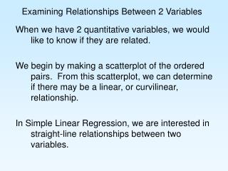
Power models Relationships between categorical variables. Exponential and Power Transformations for achieving linearity. Exponential data benefits from taking the logarithm of the response variable. Power models may benefit from taking the logarithm of both variables. y = ax p.

E N D
Power models Relationships between categorical variables
Exponential and Power Transformationsfor achieving linearity • Exponential data benefits from taking the logarithm of the response variable. • Power models may benefit from taking the logarithm of both variables.
y = axp Power law models When do we see power models? Area Volume Abundance of species
The theory behind logarithms makes it that taking the logarithm of both variables in a power model yields a linear relationship between log x and log y. Power regression models are appropriate when a variable is proportional to another variable to a power. Power Law Models y = axp
Notice the power p in the power law becomes the slope of the straight line that links logx to logy. Power Law Models y = axp yields logy= loga + plogx We can even roughly estimate what power p the law involves by finding the LSRL of logy on logx and using the slope of the line as an estimate of the power.
Body and brain weight of 96 species of mammals • You might remember this example from last time.
When we plot the logarithm of brain weight against the logarithm of body weight for all 96 species we get a fairly linear form. This suggests that a power law governs this relationship.
Bigfoot is estimated to weigh about 280 pounds or 127 kilograms. Use the model to predict Bigfoot's brain weight. Prediction from a power model
Use an inverse transformation to find the model that fits the original data. Inverse Transformation for a Power Model
Predict Xena's period of revolution from the data if it is 9.5 billion miles from the sun. What's a planet anyway?
Graphs: Scatterplot, Linearized plot, Residual plot Numerical summaries: r and r2 Model:Give an equation for our linear model with a statement of how well it fits the data Interpretation: Is our model sufficient for making predictions? Predict Xena's period of revolution (an astronomical unit is 93 million miles) What's a planet anyway?
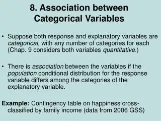
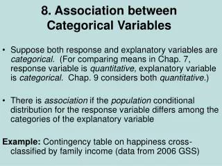
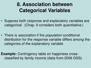
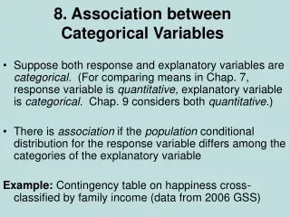
College Students • Two way table • Row variable • Column variable
College Students • Marginal distributions • Round off error
College Students • percents • Calculate the marginal distribution of age group in percents.
College Students • Each marginal distribution from a two-way table is a distribution for a single categorical variable. • Construct a bar graph that displays the distribution of age for college students.
College Students • To describe relationships among or compare categorical variables, calculate appropriate percents.
College Students • Conditional distributions • Compare the percents of women in each age group by examining the conditional distributions. • Find the conditional distribution of gender, given that a student is18 to 24 years old.