8. Association between Categorical Variables
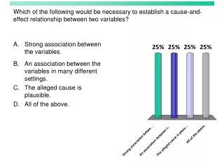
160 likes | 412 Vues
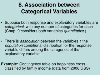
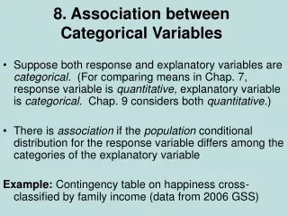
8. Association between Categorical Variables. Suppose both response and explanatory variables are categorical, with any number of categories for each ( Chap. 9 considers both variables quantitative .)

8. Association between Categorical Variables
E N D
Presentation Transcript
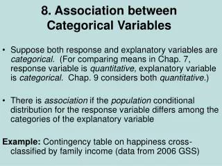
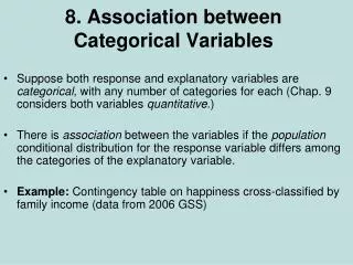
8. Association between Categorical Variables • Suppose both response and explanatory variables are categorical, with any number of categories for each (Chap. 9 considers both variables quantitative.) • There is association between the variables if the population conditional distribution for the response variable differs among the categories of the explanatory variable. • Example: Contingency table on happiness cross-classified by family income (data from 2006 GSS)
Happiness Income Very Pretty Not too Total --------------------------------------------- Above 272 (44%) 294 (48%) 49 (8%) 615 Average 454 (32%) 835 (59%) 131 (9%) 1420 Below 185 (20%) 527 (57%) 208 (23%) 920 ---------------------------------------------- • Response: Happiness • Explanatory: Level of family income • The sample conditional distributions on happiness vary by income level • Two questions: • Can we conclude that this is also true in the population? • Is the association strong or weak?
Analysis of Contingency Tables • Show sample conditional distributions: Percentages for the response variable within the categories of the explanatory variable. • Clearly define variables and categories. • If you show percentages but not the cell counts, include explanatory total sample sizes, so reader can (if desired) recover all the cell count data. • It is common to use rows for the explanatory variable and columns for response variable.
Independence & Dependence • Statistical independence (no association): Populationconditional distributions on one variable the same for all categories of the other variable • Example of statistical independence: Happiness Income Very Pretty Not too ----------------------------------------- Above 32% 55% 13% Average 32% 55% 13% Below 32% 55% 13% • Statistical dependence (association): Population conditional distributions are not all identical. • Problem: 8.3
Chi-Squared Test of Independence • Tests H0: The variables are statistically independent Ha: The variables are statistically dependent • Intuition behind test statistic: Summarize differences between observed cell counts and expected cell counts (what is expected if H0 true) • Notation: fo= observed frequency (cell count) fe= expected frequency r = number of rows in table, c = number of columns
Expected frequencies (fe): • Have same marginal distributions (row and column totals) as observed frequencies • Have identical conditional distributions. Those distributions are same as the column (response) marginal distribution of the data. • Computed by fe = (row total)(column total)/n
Happiness Income Very Pretty Not too Total -------------------------------------------------- Above 272 (189.6) 294 (344.6) 49 (80.8) 615 Average 454 (437.8) 835 (795.8) 131 (186.5) 1420 Below 185 (283.6) 527 (515.6) 208 (120.8) 920 -------------------------------------------------- Total 911 1656 388 2955 • e.g., first cell has fe= 615(911)/2955 = 189.6. • fe values are in parentheses in this table • Problem: 8.7, 8.9,
Chi-Squared Test Statistic • Summarize closeness of {fo} and {fe} by where sum is taken over all cells in the table. • When H0 is true, sampling distribution of this statistic is approximately (for large n) the chi-squared probability distribution.
Properties of chi-squared distribution • On positive part of line only • Skewed to right (more bell-shaped as df increases) • Mean and standard deviation depend on size of table through df = (r – 1)(c – 1) = mean of distribution where r = number of rows, c = number of columns • Larger values incompatible with H0,so P-value = right-tail probability above observed test statistic value.
Example: Happiness and family income df= (3 – 1)(3 – 1) = 4. P-value = 0.000 (rounded, often reported as P < 0.001). Chi-squared percentile values for various right-tail probabilities are in table on text p. 594. There is very strong evidence against H0: independence (If H0 were true, prob. would be < 0.001 of getting this large a 2 test statistic or even larger). For significance level = 0.05 (or = 0.01 or = 0.001), we reject H0 and conclude that an association exists between happiness and income.
Comments about chi-squared test • Using chi-squared dist. to approx the actual sampling dist. of the - test statistic works well for “large” random samples. Here,”large” means all or nearly all fe≥ 5. • df = (r – 1)(c - 1) means that for given marginal counts, a block of size (r – 1)(c – 1) cell counts determines the other counts.
For 2-by-2 tables, chi-squared test of independence (which has df = 1) is equivalent to testing H0: 1 = 2 for comparing two population proportions, 1 and 2 . Response variable Group Outcome 1 Outcome 2 1 1 1 - 1 2 2 1 -2 H0: 1 = 2 is equivalent to H0: response variable independent of group variable Then, Pearson 2 statistic is square of z test statistic, z = (difference between sample proportions)/(se0).
Example (from Chap. 7): College Alcohol Study conducted by Harvard School of Public Health “Have you engaged in unplanned sexual activities because of drinking alcohol?” 1993: 19.2% yes of n = 12,708 2001: 21.3% yes of n = 8783 Results refer to 2-by-2 contingency table: Response Year Yes No Total 1993 2440 10,268 12,708 2001 1871 6912 8783 Pearson 2= 14.3, df = 1, P-value = 0.000 (actually 0.00016) Corresponding z test statistic = 3.78, has (3.78)2 = 14.3.
Limitations of the chi-squared test • The chi-squared test merely analyzes the extent of evidence that there is an association. • Does not tell us the nature of the association (standardized residuals are useful for this) • Does not tell us the strength of association. • e.g., a large chi-squared test statistic and small P-value indicates strong evidence of association but not necessarily a strong association. (Recall statistical significance not the same as practical significance.)