Course Outline
430 likes | 453 Vues
This course provides a comprehensive overview of maximum-likelihood and Bayesian parameter estimation techniques for pattern classification. Topics covered include supervised learning, parametric and nonparametric approaches, density estimation, and cluster analysis.

Course Outline
E N D
Presentation Transcript
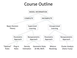
Course Outline MODEL INFORMATION COMPLETE INCOMPLETE Bayes Decision Theory Supervised Learning Unsupervised Learning Parametric Approach Nonparametric Approach Parametric Approach Nonparametric Approach “Optimal” Rules Plug-in Rules Density Estimation Geometric Rules (K-NN, MLP) Mixture Resolving Cluster Analysis (Hard, Fuzzy)
Two-dimensional Feature Space Supervised Learning
Introduction Maximum-Likelihood Estimation Bayesian Estimation Curse of Dimensionality Component analysis & Discriminants EM Algorithm Chapter 3:Maximum-Likelihood & Bayesian Parameter Estimation
Introduction • Bayesian framework • We could design an optimal classifier if we knew: • P(i) : priors • P(x | i) : class-conditional densities Unfortunately, we rarely have this complete information! • Design a classifier based on a set of labeled training samples (supervised learning) • Assume priors are known • Need sufficient no. of training samples for estimating class-conditional densities, especially when the dimensionality of the feature space is large Pattern Classification, Chapter 3 1
Assumption about the problem: parametric model of P(x | i) is available • Assume P(x | i) is multivariate Gaussian P(x | i) ~ N( i, i) • Characterized by 2 parameters • Parameter estimation techniques • Maximum-Likelihood (ML) and Bayesian estimation • Results of the two procedures are nearly identical, but there is a subtle difference Pattern Classification, Chapter 3 1
In ML estimation parameters are assumed to be fixed but unknown! Bayesian parameter estimation procedure, by its nature, utilizes whatever prior information is available about the unknown parameter • MLE: Best parameters are obtained by maximizing the probability of obtaining the samples observed • Bayesian methods view the parameters as random variables having some known prior distribution; How do we know the priors? • In either approach, we use P(i | x) for our classification rule! Pattern Classification, Chapter 3 1
Maximum-Likelihood Estimation • Has good convergence properties as the sample size increases; estimated parameter value approaches the true value as n increases • Simpler than any other alternative technique • General principle • Assume we have c classes and P(x | j) ~ N( j, j) P(x | j) P (x | j, j), where Use class j samples to estimate class j parameters Pattern Classification, Chapter 3 2
Use the information in training samples to estimate = (1, 2, …, c); i (i = 1, 2, …, c) is associated with the ith category • Suppose sample set D contains n iid samples, x1, x2,…, xn • ML estimate of is, by definition, the value that maximizes P(D | ) “It is the value of that best agrees with the actually observed training samples” Pattern Classification, Chapter 3 2
Optimal estimation • Let = (1, 2, …, p)t and be the gradient operator • We define l() as the log-likelihood function l() = ln P(D | ) • New problem statement: determine that maximizes the log-likelihood Pattern Classification, Chapter 3 2
Set of necessary conditions for an optimum is: l = 0 Pattern Classification, Chapter 3 2
Example of a specific case: unknown • P(x | ) ~ N(, ) (Samples are drawn from a multivariate normal population) = , therefore the ML estimate for must satisfy: Pattern Classification, Chapter 3 2
Multiplying by and rearranging, we obtain: which is the arithmetic average or the mean of the samples of the training samples! Conclusion: Given P(xk | j), j = 1, 2, …, c to be Gaussian in a d-dimensional feature space, estimate the vector = (1, 2, …, c)t and perform a classification using the Bayes decision rule of chapter 2! Pattern Classification, Chapter 3 2
ML Estimation: • Univariate Gaussian Case: unknown & = (1, 2) = (, 2) Pattern Classification, Chapter 3 2
Summation: Combining (1) and (2), one obtains: Pattern Classification, Chapter 3 2
Bias • ML estimate for 2 is biased • An unbiased estimator for is: Pattern Classification, Chapter 3 2
Bayesian Estimation (Bayesian learning approach for pattern classification problems) • In MLE was supposed to have a fixed value • In BE is a random variable • The computation of posterior probabilities P(i | x) lies at the heart of Bayesian classification • Goal: compute P(i | x, D) Given the training sample set D, Bayes formula can be written Pattern Classification, Chapter 1 3
To demonstrate the preceding equation, use: Pattern Classification, Chapter 1 3
Bayesian Parameter Estimation: Gaussian Case Goal: Estimate using the a-posteriori density P( | D) • The univariate Gaussian case: P( | D) is the only unknown parameter 0 and 0 are known! Pattern Classification, Chapter 1 4
Reproducing density The updated parameters of the prior: Pattern Classification, Chapter 1 4
The univariate case P(x | D) • P( | D) has been computed • P(x | D) remains to be computed! It provides: Desired class-conditional density P(x | Dj, j) P(x | Dj, j) together with P(j) and using Bayes formula, we obtain the Bayesian classification rule: Pattern Classification, Chapter 1 4
Bayesian Parameter Estimation: General Theory • P(x | D) computation can be applied to any situation in which the unknown density can be parametrized: the basic assumptions are: • The form of P(x | ) is assumed known, but the value of is not known exactly • Our knowledge about is assumed to be contained in a known prior density P() • The rest of our knowledge about is contained in a set D of n random variables x1, x2, …, xn that follows P(x) Pattern Classification, Chapter 1 5
The basic problem is: “Compute the posterior density P( | D)” then “Derive P(x | D)” Using Bayes formula, we have: And by independence assumption: Pattern Classification, Chapter 1 5
Problem of Insufficient Data • How to train a classifier (e.g., estimate the covariance matrix) when the training set size is small (compared to the number of features) • Reduce the dimensionality • Select a subset of features • Combine available features to get a smaller number of more “salient” features. • Bayesian techniques • Assume a reasonable prior on the parameters to compensate for small amount of training data • Model Simplification • Assume statistical independence • Heuristics • Threshold the estimated covariance matrix such that only correlations above a threshold are retained.
Practical Observations • Most heuristics and model simplifications are almost surely incorrect • In practice, however, the performance of the classifiers base don model simplification is better than with full parameter estimation • Paradox: How can a suboptimal/simplified model perform better than the MLE of full parameter set, on test dataset? • The answer involves the problem of insufficient data
Curve Fitting Example (contd) • The example shows that a 10th-degree polynomial fits the training data with zero error • However, the test or the generalization error is much higher for this fitted curve • When the data size is small, one cannot be sure about how complex the model should be • A small change in the data will change the parameters of the 10th-degree polynomial significantly, which is not a desirable quality; stability
Handling insufficient data • Heuristics and model simplifications • Shrinkage is an intermediate approach, which combines “common covariance” with individual covariance matrices • Individual covariance matrices shrink towards a common covariance matrix. • Also called regularized discriminant analysis • Shrinkage Estimator for a covariance matrix, given shrinkage factor 0 < < 1, • Further, the common covariance can be shrunk towards the Identity matrix,
Introduction • Real world applications usually come with a large number of features • Text in documents is represented using frequencies of tens of thousands of words • Images are often represented by extracting local features from a large number of regions within an image • Naive intuition: more the number of features, the better the classification performance? – Not always! • There are two issues that must be confronted with high dimensional feature spaces • How does the classification accuracy depend on the dimensionality and the number of training samples? • What is the computational complexity of the classifier?
Statistically Independent Features • If features are statistically independent, it is possible to get excellent performance as dimensionality increases • For a two class problem with multivariate normal classes , and equal prior probabilities, the probability of error is where the Mahalanobis distance is defined as
Statistically Independent Features • When features are independent, the covariance matrix is diagonal, and we have • Since r2 increases monotonically with an increase in the number of features, P(e) decreases • As long as the means of features in the differ, the error decreases
Increasing Dimensionality • If a given set of features does not result in good classification performance, it is natural to add more features • High dimensionality results in increased cost and complexity for both feature extraction and classification • If the probabilistic structure of the problem is completely known, adding new features will not possibly increase the Bayes risk
Curse of Dimensionality • In practice, increasing dimensionality beyond a certain point in the presence of finite number of training samples often leads to lower performance, rather than better performance • The main reasons for this paradox are as follows: • the Gaussian assumption, that is typically made, is almost surely incorrect • Training sample size is always finite, so the estimation of the class conditional density is not very accurate • Analysis of this “curse of dimensionality” problem is difficult
A Simple Example • Trunk (PAMI, 1979) provided a simple example illustrating this phenomenon. N: Number of features
Case 1: Mean Values Known • Bayes decision rule:
Case 2: Mean Values Unknown • m labeled training samples are available POOLED ESTIMATE Plug-in decision rule
Component Analysis and Discriminants • Combine features in order to reduce the dimension of the feature space • Linear combinations are simple to compute and tractable • Project high dimensional data onto a lower dimensional space • Two classical approaches for finding “optimal” linear transformation • PCA (Principal Component Analysis) “Projection that best represents the data in a least- square sense” • MDA (Multiple Discriminant Analysis) “Projection that best separatesthe data in a least-squares sense” Pattern Classification, Chapter 1 8