
Graphs
E N D
Presentation Transcript
Graphs 15-211 Fundamental Data Structures and Algorithms Ananda Gunawardena April 4, 2006
In this lecture • concept • Representations • Adjacency matrix • Adjacency List • Graph Traversals • BFS, DFS • Minimum Spanning Trees • Search Engines
Definition • Graph G = <V,E> • Set V of vertices (nodes) • Set E of edges • Elements of E are pair (v,w) where v,w V. • An edge (v,v) is a self-loop. (Usually assume no self-loops.) • Weighted graph • Elements of E are ((v,w),x) where x is a weight. • Directed graph (digraph) • The edge pairs are ordered • Undirected graph (ugraph) • The edge pairs are unordered • E is a symmetric relation • (v,w) E implies (w,v) E • In an undirected graph (v,w) and (w,v) are the same edge
Paths and cycles • A path is a sequence of nodes v1, v2, …, vN such that (vi,vi+1)E for 0<i≤N • The length of the path is N-1. • Simple path: all vi are distinct, 0<i ≤ N • A cycle is a path such that v1=vN • An acyclic graph has no cycles • A graph is connected if • given any two vertices vi and vj there exists A path from vi to vj figure 14.1 A directed graph
Vertices (aka nodes) Edges A weighted Graph BOS 618 DTW SFO 2273 211 190 PIT 318 JFK 1987 344 2145 2462 LAX Weights (Undirected)
Applications of directed graphs • Many of the common applications of graphs use directed graphs. • Often this occurs when the edges represent an asymmetric relationship. • E.g., the inheritance relationship between classes. • E.g., scheduling constraints.
Example: Course prerequisites 15-111 21-127 15-211 15-251 15-212 15-213 15-312 15-411 15-462 15-412 15-451
Example: Construction plan Building permit Pour foundation Framing Electrical wiring Plumbing Paint exterior Paint interior
Graph Density • Max number of edges in a digraph with n vertices • Max number of edges in a ugraph with n vertices?
Dense Graphs vs Sparse Graphs • A dense graph is a graph where the number of edges is relatively large compared to number of nodes • When is a graph a dense graph? • We could use • |E| = O(|V|2) - Dense • |E| = O(|V|) - Sparse • Examples of • Dense Graphs • Each node is connected to at least 25% of other nodes • Sparse Graphs • Each node is connected to only a constant number of other nodes
Relevance of a Node • Suppose G =<V,E> is a digraph and u is a vertex in V. Then • indegree(u) = {v | (v,u) in E} • That is, number of links into node u • outdegree(u) = {v | (u,v) in E} • i.e. number of links out of u
Finding indeg and outdeg • Find the indegree and outdegree for each of the nodes
1 2 3 4 5 6 7 1 x x 2 x x 3 x 4 x x x 1 2 5 x x 3 6 4 7 5 1 2 6 3 4 7 4 5 3 4 5 6 3 6 7 4 7 6 7 Representing graphs • Adjacency matrix • Adjacency lists
Implementing Adjacency List figure 14.4
Graph Representations • Draw the adjacency matrix and list representations of the following digraph (unweighted).
1 2 3 4 5 6 7 1 x x 2 x x 3 x 4 x x x 1 2 5 x x 3 6 4 7 5 6 3 4 7 4 5 6 3 6 7 4 7 Space Complexity • Memory Requirements for • Adjacency List – O(|V|+|E|) • Adjacency Matrix – O(|V|2) • We can reduce the memory requirements by using “packed” arrays
Time Complexity • Query: Does (u,v) Є E ? • Time complexity depends on graph representation • Adjacency list – O(|V|+|E|) • Adjacency matrix – O(1)
Reversing a Graph • Suppose Gr = <V, Er> where (u,v) in E if and only if (v,u) is in Er • Example: Let G = {(1,2), (2,3), (3,1)}, then Gr = { } • Give an algorithm to compute Gr • If G is represented as adjacency matrix • If G is represented as adjacency list • What is the complexity of your algorithm in each case?
Trees are graphs • A dag is a directed acyclic graph • A forest is a dag in which every node has indegree at most 1. • A tree is a forest with exactly one root.
Detecting Cycles BOS DTW SFO PIT JFK LAX How do you detect a cycle in a graph?
Reachability • Given a node u in V, find all the nodes v in V that are reachable from u. That is, find the set • R(u) = {v|There is a path from u to v} • How do we compute R(u)? • u is in R(u) – trivial or base case • If v is in R(u) and (v,z) in E, then z is in R(u) • So we can inductively find the set R(u)
Reachability Algorithms • There are two algorithms • Depth First Search (DFS) • Explore the nodes by going deeper and deeper into the graph. Use back tracking to try different paths (uses a stack) • Breadth First Search (BFS) • Explore the nodes in an orderly manner. Look at the nodes that are closest to source. Then look at their neighbors, etc.. (uses a queue)
DFS Algorithm • Let R be the set of vertices reachable from starting node x, let S be a stack DFS(vertex x) S.push(x); put x into R while (S is not empty) u = S.pop(); for all (u,y) in E { if y is not in R put y into R S.push(y) } } // end while
Recursively DFS(vertex x) { put x into R; for all (x,y) in E do if (y is not in R) DFS(y); }
When does a graph has a cycle? • If every node in a graph has out-degree at least 1, then the graph has a cycle. • Proof: (informally) Start from any node and walk through the graph • Since you can go out from any node, you can touch all the nodes and eventually you will run into a node that you have already visited. • So that is a cycle. • We can make similar statement about in-degree
Finding a Cycle • We can do DFS to traverse the graph • We can use colors to keep track of • Nodes that are not visited • Nodes we are visiting now • Nodes that are already visited
Example DFS(1) DFS(2) DFS(7)DFS(3)DFS(4)DFS(5) If DFS runs into a node still visiting, then we have a cycle
Breadth First Search (BFS) BFS (node x){ Q.enque(x) ; // assume Q is a Queue put x into R; // R is the set of vertices visited in BFS while (Q is not empty) u = Q.deque(); for all neighbors v of u if v is not in R put v into R Q.enque(v);
Homework • Perform BFS starting from 1. Show the state of the queue and nodes visited at each stage.
Problem: Laying Telephone Wire Central office
Wiring: Naïve Approach Central office Expensive!
Wiring: Better Approach Central office Minimize the total length of wire connecting the customers
Minimum Spanning Tree (MST) (see Weiss, Section 24.2.2) A minimum spanning tree is a subgraph of an undirected weighted graph G, such that • it is a tree (i.e., it is acyclic) • it covers all the vertices V • contains |V| - 1 edges • the total cost associated with tree edges is the minimum among all possible spanning trees • not necessarily unique
9 b 9 b a 6 2 a 6 2 d d 4 5 4 5 5 4 5 4 e 5 e 5 c c How Can We Generate a MST?
9 b a 6 2 d 4 5 5 4 e 5 c e a b c d 0 Prim’s Algorithm Initialization a. Pick a vertex r to be the root b. Set D(r) = 0, parent(r) = null c. For all vertices v V,v r, set D(v) = d. Insert all vertices into priority queue P, using distances as the keys Vertex Parent e -
Prim’s Algorithm While P is not empty: 1. Select the next vertex u to add to the tree u = P.deleteMin() 2. Update the weight of each vertex w adjacent to u which is not in the tree (i.e., w P) If weight(u,w)< D(w), a. parent(w) = u b. D(w) = weight(u,w) c. Update the priority queue to reflect new distance for w
d b c a 4 5 5 Prim’s algorithm Vertex Parent e - b e c e d e 9 b a 6 2 d 4 5 5 4 e 5 c The MST initially consists of the vertex e, and we update the distances and parent for its adjacent vertices
Prim’s algorithm Vertex Parent e - b e c d d e a d 9 b a 6 2 d 4 5 5 4 e 5 c The final minimum spanning tree
Prim’s Algorithm Invariant • At each step, we add the edge (u,v) s.t. the weight of (u,v) is minimum among all edges where u is in the tree and v is not in the tree • Each step maintains a minimum spanning tree of the vertices that have been included thus far • When all vertices have been included, we have a MST for the graph!
Initialization of priority queue (array): O(|V|) • Update loop: |V| calls • Choosing vertex with minimum cost edge: O(|V|) • Updating distance values of unconnected vertices: each edge is considered only once during entire execution, for a total of O(|E|) updates • Overall cost without heaps: • What is the run time complexity if heaps are used? O(|E| + |V|2)) Running time of Prim’s algorithm(without heaps)
Correctness • Lemma: Let G be a connected weighted graph and T be a MST. Let G’ be a subgraph of T. Let C be a component of G’ .Let S be the set of all edges with one vertex in C and other not in C. If we add a minimum edge weight in S to G’, then the resulting graph is contained in a minimal spanning tree of G
Correctness • Theorem: Prim’s algorithm correctly finds a minimal spanning tree • Proof: by induction show that tree constructed at each iteration is contained in a MST. Then at the termination, the tree constructed is a MST • Base case: tree has no edges, and therefore contained in every spanning tree • Inductive case: Let T be the current tree constructed using Prim’s algorithm. By inductive argument, T is contained in some MST. • Let (u,v) be the next edge selected by Prim’s, such that u in T and v not in T. Let G’ be T together with all vertices not in T. Then T is a component of G’ and (u,v) is a minimum weight edge with one vertex in T and one not in T. Then by lemma, when (u,v) is added to G’ , the resulting graph is also contained in a MST.