The zero bound to nominal interest rates
800 likes | 997 Vues
The zero bound to nominal interest rates. Lectures to MSc Advanced Macro, Bristol, Spring 2014 Tony Yates. 1. Zero bound: introduction. Policy rates across the world. Source: Stone et al , IMF, 2011. Source: Natixis special report by Sylvain Broyer, Feb 27, no 30.

The zero bound to nominal interest rates
E N D
Presentation Transcript
The zero bound to nominal interest rates Lectures to MSc Advanced Macro, Bristol, Spring 2014 Tony Yates
Policy rates across the world Source: Stone et al, IMF, 2011
Source: Natixis special report by Sylvain Broyer, Feb 27, no 30. As room for conventional stimulus ran out at the zero bound... Central banks bloated their balance sheets as they engaged in unconventional stimulus of one sort or another.
Overview: 4 examinable topics • Why does the zero bound exist? • Analytical study of money demand • What computational challenges does it pose for us as economists? • Multiple non linear rational expectations equilibria • What have central banks done about it? • Forward guidance • Quantitative and credit easing • What else could they do about it? • Currency reform to allow negative interest rates
Useful sources and reading • McCallum, ‘Theoretical analysis regarding the ZLB…’ • Brendon et al ‘The pitfalls of speed-limit interest rate rules at the ZLB’ • Miles Kimball blog [various besides this link] • Yates ‘The zero bound…’: BoE version, ECB version • Goodfriend: ‘Overcoming the zero bound…’
Useful sources/ctd… • Walsh’s text book • Eggertson and Woodford • New monetarist economics surveys on models and methods [linked to later in slides] • Willem Buiter on –ve rates • ‘Unconventional monetary policy: lessons from the past 3 years’, FRBSF, speech.
Useful sources/ctd… • 'Methods of policy accommodation at the interest-rate lower bound', [Jackson Hole lecture] • 'The central bank balance sheet as an instrument of monetary policy' [with Curdia] • ‘Macroeconomic effects of FOMC forward guidance’, Charles Evans et al • “The other imbalance and the financial crisis”, Ricardo Caballero (2009), http://www.nber.org/papers/w15636 • ‘A model of the safe asset mechanism: safety traps and economic policy’, Caballero and Farhi (2012) • The aggregate demand for Treasury debt, Vissing-Jorgensen and Krishnamurthy • ‘A Modigliani-Miller theorem for OMOs’, Wallace
Even more useful sources. • ‘The effects of QE on long term interest rates’,Vissing-Jorgensen and Krishnamurthy • ‘The UK’s QE policy’, Joyce et al... • ‘QE and unconventional monetary policy – an introduction’, Joyce, Miles, Scott, Vayanos [EJ conference volume].
Why the zero bound exists: McCallum Consumer’s objectives Sequence of constraints faced by consumers. Function determining transactions costs associated with consumption. Crucial part of the story of the zero bound.
Existence of zero bound/ctd… The Lagrangian. We will differentiate wrt real balances, m, and bonds, b. FONCs are application of Kuhn-Tucker.
Existence of zero bound/ctd… Write out two elements in the infinite Lagrangian sum, to trace out where m_t and b_t enter. Presence of dated ‘t+1’ elements means, eg, that m_t enters the time t and the time t-1 elements in this infinite sum….
FOCs for m_t,b_t We combine these two equations to get the one below, linking the nominal rate to the partial derivative of this transactions function. Since the p.d. is assumed to be always<0, the RHS is always >0. However, if at some point there were resource costs of ‘storing’ real balances, this p.d. could turn positive [more balances are counterproductive] and therefore the nominal rate cd be <0.
Money demand and the zero bound • Liquidity services value of real balances declines as liquidity increases; • To persuade people to hold larger real balances, opportunity cost [the nominal interest rate] has to fall. • Zero bound arises because cash, which earns zero interest, dominates any –ve interest rate investment • At the zero bound, OMOs involve the swap of one zero interest, default risk-free asset for another
The tragedy and the bliss of the zero bound • At the zero bound, if it exists, we have squeezed the marginal reduction in transactions costs associated with holding money to zero. This is good. This is the Friedman Rule. • But, we have also run out of room to use interest rates to counter-act negative shocks to the natural rate of interest.
Tragedy and bliss of the zero bound/ctd… • How costly this is depends on how costly are fluctuations in inflation and real variables. • And how effective are substitutes to interest rate policy, for example: • Traditional fiscal policy • Unconventional monetary policy • Usually given as a reason to choose positive steady state inflation rates. Absent shocks, optimal inflation rate in NK model determined by Friedman Rule vs price stickiness.
Money demand and the zero lower bound • We used ‘transactions costs’ formulation of money demand. • Elsewhere [eg McCallum and Goodfriend] referred to as ‘shopping-time’ model of money demand • Equivalent in most respects is ‘money in the utility function’: Woodford’s NK model is the limit of this model as the MIU parameter tends to zero. • All assume the value of holding or using money.
New monetarist economics • Kiyotaki-Wright, Lagos-Wright, Williamson-Wright and others. • Derive valued money in search equilibrium. • View NK MIU/ST/CIA models as suspect. Assumed value of money contradicts otherwise fricitonless trade model. • Some common results, eg optimality of Friedman Rule. • See methods and models surveys.
3. A baby, nonlinear rational expectations, perfect foresight model of interest rates at the ZLB
REE, the zlb, computation, nonlinearities, multiplicity • Zero bound makes policy rule nonlinear, invalidating linear RE methods. • Full nonlinear RE tricky, computationally challenging, sometimes infeasible for rich, realistic models. • Because rates are fixed, there is the spectre of multiplicity [maybe you encountered this with the ‘Taylor Principle’ in Engin’s course?]
In brief • ‘Speed-limit’ rule: • Self-fulfilling recessions at the ZLB • Two examples: • Feeding back on growth, in a simple NK model • ...house price growth in Iacoviello (2005)
Why are speed-limit rules of interest? • Implement/mimic commitment policy • Walsh(2003a), Giannoni and Woodford (2003), McCallum and Nelson(2004), Stracca (2007), Leduc and Natal(2011) • Blake (2011) • Insurance against measurement error • Orphanides and Williams [various]) • Some evidence they fit time series for central bank rates • Mehra (2002)
Speed limit rules and commitment • Optimal policy involves history-dependence • Responding to rates of change confers that history dependence
Speed limit rules and measurement error [Stolen from Walsh FRBSF Economic Letter, 2003]
Solution method • ‘Piecewise-linear’, perfect foresight RE • Jung, Teranishi and Watanabe (2005), Eggertson and Woodford (2003) • Simple, not optimal policy • Guess period at which ZLB binds; solve resultant, 2 part linear system, verify whether we have an REE
RE solution concepts • Perfect foresight means: agents literally see the future, exactly. • RE: agents can’t anticipate future shocks, but can ‘solve the model’ for expectations, and use the reduced form to forecast future variables conditional on already observed shocks.
Pros and cons of perfect foresight • Pros: • Greatly simplifies solution method. Can solve larger, more realistic models [ie aside from assumption about expectations] and more quickly and accurately. • For some questions perhaps it’s ok to assume perfect foresight. Egagents indifferent to risk, or studying some pre-announced policy.
Pros and cons of perfect foresight • Cons • Few questions for which agents literally can see the future. • And agents probably do care about risk enough for it to matter. Uncertainty about future weighs down on current spending. • Zero bound likely a time of heightened risk, and high risk intolerence?
Solution algorithm 1. Guess ZLB binds at t=0, but not thereafter. 2. Conventional RE solvers give us: 3. Now solve for initial period, substituting out expectations using 2.: 4. Given initial values, use 2. to solve recursively for t=1 onwards... 5. Verify:
Recap on nonlinear ZLB solution method in words • Make a guess at the number of periods for which the zero bound binds. • Use undetermined coefficients or similar to solve for linear REE in terms of state from this period on. • Use this solution form to eliminate the expectations terms in the equation system for the initial period. • This leaves you with a 2-equation 2 unknown system for the initial period, which you can solve. Remember that the interest rate rule is replaced by the assumption that interest rates are zero (from the initial guess). • Having solved for the initial period, use the solution form for the post zero bound period to simulate forwards step by step.
Dynamics under self-fulfilling recession • Inflation and output >4% from ss • Rates at the ZLB
Real rate under self-fulfilling recession Real rate high in period 2, sustaining forecast of low inflation and output.
Intuition for self fulfilling recession • Rates at the ZLB implies inflation and output low • Inflation and output low implies forecasts of () low • Forecasts low implies policy forecast to be tight tomorrow • Policy tight tomorrow if speed limit motivates preventing a bounce back in activity
Why we need ZLB and speed limits • Without ZLB, Taylor principle rules out initial fall in output as an REE • Without concern for growth rates, forecast of future policy too loose to sustain low values for inflation and output in the future... • Therefore initial values for inflation and output not low enough to take rates to the ZLB.
Analytical conditions for sunspots When we set gives sunspots For Necessary but not sufficient condition for sunspots is Eg Sunspots occur provided
Conditions for sunspots When we set gives sunspots For Sunspots occur provided
Example 2: feeding back off house prices in the Iacoviello model • Why bother with this example? • How general is pathology of speed limit rules? • Central banks have been urged to pay more attention to asset prices • Measurement error/commitment logic applies to asset prices too
Iacoviello (2005)/[KM, 1998] • Consumers: • patient, • consume goods and housing services, • supply labour to entrepreneurs • Entrepreneurs: • Impatient • Produce, using commercial property as a factor • Borrow against value of property, up to a fixed fraction
Self-fulfilling recessions in Iacoviello’s model • Moderate recession in output, >3pp below ss • House prices around 5pp below ss
Feeding back from credit growth in Iacoviello’s model • Crisis has raised credit growth as a concern, so plausible candidate for inclusion in a policy rule • These rules also generate self-fulfilling recessions. • Eg: ...is sufficient to deliver self-fulfilling recessions
Indeterminacy: discussion • Benhabib, Schmitt-Grohe and Uribe (2002): • Global indeterminacy • 2 steady states: good one, liquidity trap • Mertens and Ravn (2011) • Shocks to expectations functions • Switches in beliefs about ss to which economy is converging • Liquidity trap provoked by belief that there will be one • Our paper • local indeterminacy • Convergence to desirable steady state • Only 2 equilibria, not many. Either recession, or nothing.
Remarks • Can we get persistent ZLB episodes? • Yes and no • Allowing for interest rate inertia • Still get sunspots • Only ‘2’, not infinite numbers of self-fulfilling expectationalequilibria • Survives analysis of the full nonlinear model, not just the quasi-linear approximation used here.
Recap [on speed limits] • Speed limit rules can lead to self-fulfilling recessions • Examples with output, house price and credit growth • Weighs against other motives for these rules (measurement error, mimicking commitment) • Property only of RE models; requires that other instruments can’t circumvent ZLB
Recap [on conceptual learning points in speed limits paper] • Perfect foresight, ‘quasi-linear’ RE. • Benefits: tractability, cd handle big model. • Costs: realism. We don’t see the future. • Analagous method used by EgWd to solve for optimal monetary policy. • Multiplicity=multiple links between observables and fundamentals.
Recap on zero bound lecture • Analytical derivation of the conditions under which zero bound exists. • Demonstration of computational challenge posed by the ZLB, and the economic pathologies it can generate.
What we haven’t yet covered that you may be examined on • Quantitative easing; effects and criticisms • Eggertson and Woodford’s optimal monetary policy at the ZLB, and how it compares to central bank ‘forward guidance’. • Credit easing. • Other options at the zero bound – eg currency reform to allow negative interest rates. • These topics may come up as essay questions I the exam or resit. • Some of these topics may be recapped on in an open lecture to you and undergrads. • With essay topics, don’t assume that a good answer can confine itself to what we do in the lectures.