Download
1 / 29
290 likes | 375 Vues
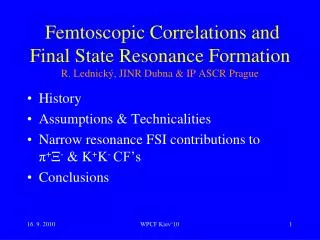
Femtoscopic Correlations and Final State Resonance Formation R. Lednický, JINR Dubna & IP ASCR Prague. History Assumptions & Technicalities Narrow resonance FSI contributions to π + - K + K - CF’s Conclusions. History. Correlation femtoscopy :.

E N D
WPCF Kiev‘10 Femtoscopic Correlations and Final State Resonance Formation R. Lednický, JINR Dubna & IP ASCR Prague • History • Assumptions & Technicalities • Narrow resonance FSI contributions to π+- K+K- CF’s • Conclusions
History Correlation femtoscopy : measurement of space-time characteristics R, c ~ fm Fermi’34:e± NucleusCoulomb FSI in β-decay modifies the relative momentum (k) distribution → Fermi (correlation) function F(k,Z,R) is sensitive to Nucleusradius R if charge Z » 1 of particle production using particle correlations
Fermi function F(k,Z,R) in β-decay F = |-k(r)|2~ (kR)-(Z/137)2 Z=83 (Bi) β- 2 fm 4 R=8 β+ k MeV/c
Modern correlation femtoscopy formulated by Kopylov & Podgoretsky KP’71-75: settled basics of correlation femtoscopy in > 20 papers (for non-interacting identical particles) • proposed CF= Ncorr /Nuncorr& mixing techniques to construct Nuncorr •showed that sufficientlysmooth momentum spectrum allows one to neglect space-time coherence at small q* |∫d4x1d4x2p1p2(x1,x2)...|2 →∫d4x1d4x2p1p2(x1,x2)|2... •clarified role of space-time characteristics in various models
Assumptions to derive “Fermi” formula for CF CF = |-k*(r*)|2 - two-particle approximation (small freezeout PS density f) ~ OK, <f> 1 ? lowpt - smoothness approximation: pqcorrel Remitter Rsource ~ OK in HIC, Rsource20.1 fm2 pt2-slope of direct particles usually OK - equal time approximation in PRF RL, Lyuboshitz’82 eq. time condition |t*| r*2 to several % - tFSI = dd/dE >tprod tFSI (s-wave) = µf0/k* k*= ½q* hundreds MeV/c • typical momentum transfer in the production process RL, Lyuboshitz ..’98 & account for coupled channels within the same isomultiplet only: +00, -p 0n, K+KK0K0, ... tFSI (resonance in any L-wave) = 2/ hundreds MeV/c
Caution: Smoothness approximation is justified for small k<<1/r0 ∫d4x1d4x2 G(x1,p1;x2,p2) |p1p2(x1,x2)|2 ∫d3r WP(r,k) |-k(r)|2 ∫d3r {WP(r,k) + WP(r,½(k-kn)) 2Re[exp(ikr)-k(r)] +WP(r,-kn) |-k(r)|2 } where-k(r) = exp(-ikr)+-k(r) andn = r/r Thesmoothness approximation WP(r,½(k-kn)) WP(r,-kn) WP(r,k) is valid if one can neglect the k-dependence of WP(r,k), e.g. for k << 1/r0
Technicalities – 2: treating the spin & angular dependence Assuming that one of the two particles is spinless and the other one is either spin-1/2 or spin-1/2, we have: Angular dependence enters only through the angle between the vectors k and r in the argument of the Wigner (rotation) d-functions.
Technicalities – 3: contribution of the outer region For r > d = the range of the strong interaction potential, the radial functions:
Technicalities – 4: projecting pair spin & isospin =π+- =K+K-
Technicalities – 8: simple Gaussian emission functions In the following we use the simple one-parameter Gaussian emission function: WP(r,k) = (8π3/2r03)-1 exp(-r2/4r02) and account for the k-dependence in the form ( = angle between r and k) WP(r,k) = (8π3/2r03)-1 exp(-b2r02k2) exp(-r2/4r02 + bkrcos) Note the additional suppression of WP(0,k) if out 0: WP(0,k) ~exp[-(out/2r0)2] (~30% suppression for π+-)
References related to resonance formation in final state: R. Lednicky, V.L. Lyuboshitz, SJNP 35 (1982) 770 R. Lednicky, V.L. Lyuboshitz, V.V. Lyuboshitz, Phys.At.Nucl. 61 (1998) 2050 S. Pratt, S. Petriconi, PRC 68 (2003) 054901 S. Petriconi, PhD Thesis, MSU ,2003 S. Bekele, R. Lednicky, Braz.J.Phys. 37 (2007) 994 B. Kerbikov, R. Lednicky, L.V. Malinina, P. Chaloupka, M. Sumbera, arXiv:0907.061v2 B. Kerbikov, L.V. Malinina, PRC 81 (2010) 034901 R. Lednicky, P. Chaloupka, M. Sumbera, in preperation
p-X correlations in Au+Au (STAR) P. Chaloupka, JPG 32 (2006) S537; M. Sumbera, Braz.J.Phys. 37(2007)925 • Coulomb and strong FSI presentX*1530, k*=146 MeV/c, =9.1 MeV • No energy dependence seen • Centrality dependence observed, quite strong in the X* region; 0-10% CF peak value CF-1 0.025 • Gaussian fit of 0-10% CF’s at k* < 0.1 GeV/c: r0=4.8±0.7 fm, out = -5.6±1.0 fm r0 =[½(rπ2+r2)]½ of ~5 fm is in agreement with the dominant rπ of 7 fm
K+ K-correlations in Pb+Pb (NA49) PLB 557 (2003) 157 • Coulomb and strong FSI present1020, k*=126 MeV/c, =4.3 MeV • Centrality dependence observed, particularly strong in the region; 0-5% CF peak value CF-1 0.10 • 3D-Gaussian fit of 0-5% CF’s: out-side-long radii of 4-5 fm
Resonance FSI contributions to π+- K+K- CF’s • Complete and corresponding inner and outer contributions of p-wave resonance (*) FSI to π+- CF for two cut parameters 0.4 and 0.8 fm and Gaussian radius of 5 fm * FSI contribution strongly overestimated • The same for p-wave resonance () FSI contributions to K+K- CF FSI contribution well described but no room for direct production ! Rpeak(STAR) 0.025 ----------- ----- Rpeak(NA49) 0.10 ----------- -----
Peak values of resonance FSI contributions to π+- K+K- CF’s vs cut parameter • Complete and corresponding inner and outer contributions of p-wave resonance (*) FSI to peak value of π+- CF for Gaussian radius of 5 fm • The same for p-wave resonance () FSI contributions to K+K- CF for < r0, CF is practically -independent at ~1 fm, CFCF(inner) Rpeak(STAR) 0.025 ----- --------------- Rpeak(NA49) 0.10 -----------------------
Angular dependence in the *-resonance region (k*=140-160 MeV/c) 0-10% 200 GeV Au+Au FASTMC-code from L. Malinina r* < 1 fm r* < 0.5 fm = angle between r and k WP(r,k) ~ exp[-r2/4r02 + b krcos] b 0.5
Angular dependence – example parametrization WP(r,k) ~ exp[-r2/4r02 + bkrcos]; = angle between r and k R(π+-) k=146 MeV/c, r0=5 fm Suppressing WP(0,k) by a factor of exp[-b2r02k2] Smoothness assumption: WP(r,½(k-kn)) WP(r,-kn) WP(r,k) Exact Rpeak(STAR) -------------- 0.025 b=0.3 0.4 Similar suppression of resonance contribution to CF b
Accounting for angular dependence:FASTMC-code (implying smoothness assumption) close to the STAR peak but too low at small k* (L.M.) OK at small k* but much higher peak (P. Ch.) b < 0.4 Indicating that the parametrization of the angular dependence ~ exp(b krcos), b0.5 is oversimplified Rpeak(STAR) -------------- 0.025
Summary • Assumptions behind femtoscopy theory in HIC seem OK, including both short-range s-wave and narrow resonance FSI up to a problem of the angular dependence in the resonance region. • The effect of narrow resonance FSI scales as inverse emission volume r0-3, compared to r0-1 or r0-2 scaling of the short-range s-wave FSI, thus being more sensitive to the space-time extent of the source. The higher sensitivity may be however disfavoured by the theoretical uncertainty in the case of a strong angular asymmetry. • The NA49 (? STAR) correlation data from the most central collisions seem to leave a little or no room for a direct (thermal) production of near threshold narrow resonances.
QS symmetrization of production amplitudemomentum correlations of identical particles are sensitive to space-time structure of the source KP’71-75 total pair spin CF=1+(-1)Scos qx exp(-ip1x1) p1 2 x1 ,nns,s x2 1/R0 1 p2 2R0 nnt,t PRF q =p1- p2 → {0,2k} x = x1- x2 → {t,r} |q| 0 CF →|S-k(r)|2 =| [ e-ikr +(-1)S eikr]/√2 |2
Final State Interaction |-k(r)|2 Similar to Coulomb distortion of -decay Fermi’34: Migdal, Watson, Sakharov, … Koonin, GKW, ... fcAc(G0+iF0) s-wave strong FSI } FSI nn e-ikr -k(r) [ e-ikr +f(k)eikr/r ] CF pp Coulomb |1+f/r|2 kr+kr F=1+ _______ + … eicAc ka } } Bohr radius Coulomb only Point-like Coulomb factor k=|q|/2 FSI is sensitive to source size r and scattering amplitude f It complicates CF analysis but makes possible Femtoscopy with nonidentical particlesK,p, .. & Coalescence deuterons, .. Study “exotic” scattering,K, KK,, p,, .. Study relative space-time asymmetriesdelays, flow
BS-amplitude For free particles relate p to x through Fourier transform: Then for interacting particles: Product of plane waves -> BS-amplitude : Production probability W(p1,p2|Τ(p1,p2;)|2
Smoothness approximation: rA« r0 (q « p) W(p1,p2|∫d4x1d4x2p1p2(x1,x2) Τ(x1,x2;)|2 =∫d4x1d4x1’d4x2d4x2’ r0 - Source radius rA - Emitter radius p1p2(x1,x2)p1p2*(x1’,x2’) Τ(x1,x2 ;)Τ*(x1’,x2’ ;) p1 x1 ≈ ∫d4x1d4x2G(x1,p1;x2,p2) |p1p2(x1,x2)|2 x1’ x2’ Source function G(x1,p1;x2,p2) = ∫d4ε1d4ε2 exp(ip1ε1+ip2ε2) Τ(x1+½ε1,x2 +½ε2;)Τ*(x1-½ε1,x2-½ε2;) x2 p2 2r0 For non-interacting identical spin-0 particles – exact result (p=½(p1+p2) ): W(p1,p2∫ d4x1d4x2 [G(x1,p1;x2,p2)+G(x1,p;x2,p) cos(qx)] approx. result: ≈ ∫d4x1d4x2 G(x1,p1;x2,p2) [1+cos(qx)] = ∫ d4x1d4x2 G(x1,p1;x2,p2) |p1p2(x1,x2)|2
Effect of nonequal times in pair cms → RL, Lyuboshitz SJNP 35 (82) 770; RL nucl-th/0501065 Applicability condition of equal-time approximation: |t*| r*2 r0=2 fm 0=2 fm/c r0=2 fm v=0.1 OK for heavy particles OK within 5% even for pions if 0 ~r0 or lower
Technicalities – 7: volume integral I(,k) In the single flavor case & no Coulomb FSI For s & p-waves it recovers the results of Wigner’55 & Luders’55