Efficient Ray Tracing of Compressed Point Clouds Using Quantized kd-Tree
This paper presents a novel approach for efficient ray tracing of large 3D models represented as compressed point clouds, utilizing a Quantized kd-Tree structure. The method addresses the challenges of rendering extensive models that exceed main memory capacity by compressing the data, thereby facilitating faster access and processing. Our solution not only improves spatial querying but also allows for a multiresolution representation, effectively balancing rendering speed and visual quality. Key applications include 3D scanning, industrial inspection, and cultural heritage preservation.

Efficient Ray Tracing of Compressed Point Clouds Using Quantized kd-Tree
E N D
Presentation Transcript
Efficient Ray Tracing of Compressed Point Clouds The Quantizedkd-Tree Erik HuboTom MertensTom HaberPhilippe Bekaert Expertise Centre for Digital Media Hasselt University
Goal: Display Large Models • 3D scanners • Industrial inspection • Preservation of cultural heritage • …
Goal: Display Large Models • How? • Use points to represent model • Compress model • Ray trace compressed model
Why Compression? • Increasing resolution of 3D scanners • Ray tracing efficient if model in main memory • Models: +100 M points > 1GB (only positions) • Model size > memory size stalls due to slow disk access • Solution? out-of-core (disk access needed) • Compression reduces model size
Our approach • Ray tracing requires local neighborhood • Caching precomputed neighborhoods? • Additional memory cost • Querying on the fly • Challenge: compression + spatial querying Moving Least Squares [Adamson and Alexa 2003,2004]
Related Work • Point-based rendering: • QSplat [Rusinkiewicz and Levoy 2000] • Sequential Point Trees [Dachsbacher 2003] • Ray-tracing point clouds • [Schaufler and Jensen 2000] • [Adamson and Alexa 2003] • [Bart Adams et al. 2005] • [Ingo Wald et al. 2005]
Related Work • Compression • 1.QSplat _ • 2.[Botsch 02] _ _ _ _ _ _ _ _ _ _ _ _ • 3.[Gandoin 02] _ • 4.[Krüger 05] _ _ _ _ _ _ _ _ _ _ _ _ • 5.[Waschbüsch 04] _ • 4.[Ochotta 04] _ _ _ _ _ _ _ _ _ _ _ _ • 7.[Gumhold 05] _ • No efficient spatial querying: • Pointers are discarded: 1,2,3,4 • Sequential full decompression: 4,5,6,7 The Quantized kd-tree: Local Decoding
1 2 3 2 3 8 1 9 4 5 6 7 4 5 6 7 8 9 Quantized kd-Tree • Left-Balanced kd-Tree [Jensen01]: • Subdivides space in 2 axis aligned box shaped regions (binary tree) • Splitting plane at median point • Splitting direction X, Y, Z
Quantized kd-Tree • Motivation for kd-Tree: + Efficient spatial querying + Efficient ray tracing [Wald 05] • Motivation for Left-Balanced kd-Tree + Stored as heap no pointers - Balancing may harm performance [Wald 04]
Quantized kd-Tree • Derived from Left-Balanced kd-Tree: • Normalized splitting plane offset d, w.r.t. current bounding box, d [0,1) and quantize d D • Leaf nodes represent input points Normal Median Split Quantized kd-Tree Median Split Quantization
0 1 0 .6 Internalnode .4 .6 .5 .6 .5 + (.6 - .5)*(7/8) = .59 Local Decoding Root leaf 3 bit per split plane – 8 quantization steps
Precision: 1D q = 8 = 23 1 0 d [0,1) • Precision depends on tree depth: L • Error decreases: • Worst: 1 • Best: 1/q (= 1 quantization step) • Avg: 0.5 < α = q+1 < 1 2q • Precision ~ αL Quant. split = q*d 1/q
Ray Ray Ray Unquantized Splitting Position Local Decoding:Quantization uncertainty • Let child bounding boxesoverlap by one quantization step • Extend tree traversaland spatial query algorithms Quantization Left Region Right Region Overlap Region This point is missed
Ray Overlap Local Decoding: The Overlap Region • Low #quantization steps Large overlap region • Top of tree: examine both subtrees! Large overhead! • E.g. q = 4 56 times slower
Fixed vs. Variable Quantization Fixed Variable 2 16 16 2 2 16 2 8 2 3 2 2 2 1 q = 2 q = 1..16 • Traversal overhead • Poor quality + Less overhead, better quality + Only small additional cost
Results Bpp: 15.5 PSNR: 79.1dB Bpp: 5.6 PSNR: 62.8 dB Bpp: 8.6 PSNR: 69.4 dB Uncompressed
Multiresolution Representation • Inner nodes represent LOD points • Median position = LOD point • Detail level based on projected screen size Level 13 Level 15 Level 18 Full
Results • Multiresolution • Rendering times are 9 times faster with LOD • Reduces aliasing artifacts: Without LOD With LOD
Camera position changed Results • Comparison of rendering times on 1 PC, 2GBRAM: • Compressed St Matthews (890 MB) : 9s • Uncompressed St Matthews (3.6 GB) : 36 …150s • In both cases normals were compressed to 12 bit Compressed Uncompressed
Results • Rendering large scenes : • 10 sec 1 PC: 512x512 374M points(without instancing) 229M points
Conclusion • Compress and display huge models • Spatial querying on compressed data • Suited for ray tracing • Multiresolution representation • Future work • Compress other attributes, e.g. normals, colors
Questions? • Acknowledgments • Stanford Scanning Repository • BOF: Bijzonder Onderzoeks Fonds • Belgian American Educational Foundation • Contact: erik.hubo@uhasselt.be http://research.edm.uhasselt.be/ehubo