Download
1 / 27
270 likes | 301 Vues
Discover lensing principles and mass reconstruction techniques in gravitational lensing, including PixeLens and Bayesian approaches. Learn about lensing plane properties, time delays, and image magnifications, with examples from galaxies and clusters.

E N D
Gravitational Lensing: Mass Reconstruction Methods and Results Liliya L.R. Williams (U Minnesota) Prasenjit Saha (QMW, London & Univ. of Zurich)
Outline Galaxy cluster Abell 1689 • Brief, non-technical introduction to strong (multiple image) lensing • Bayesian approach to the reconstruction of lens mass distribution • Overview of mass reconstruction methods and results • Non-parametric (free-form) lens reconstruction method: PixeLens • Open questions and future work
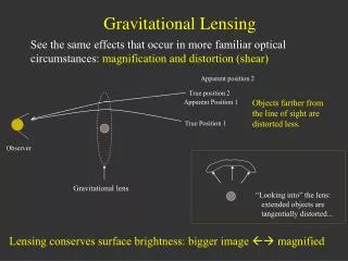
A Brief Introduction to Lensing Goal: find positions of images on the plane of the sky How? use Fermat’s Principle - images are formed at the local minima, maxima and saddle points of the total light travel time (arrival time) from source to observer position on the sky total travel time
A Brief Introduction to Lensing Plane of the sky Circularly symmetric lens On-axis source Circularly symmetric lens Off-axis source Elliptical lens Off-axis source
All the Information about Imagesis contained in the Arrival Time Surface Positions: Images form at the extrema, or stationary points (minima, maxima, saddles) of the arrival time surface. Time Delays: A light pulse from the source will arrive at the observer at 5 different times: the time delays between images are equal to the difference in the “height” of the arrival time surface. Magnifications: The magnification and distortion, or shearing of images is given by the curvature of the arrival time surface. [Schneider 1985] [Blandford & Narayan 1986]
Substructure and Image Properties Maxima, minima, saddles of the arrival time surface correspond to images smooth elliptical lens … with mass lump (~1%) added
Examples of Lens Systems Galaxy Clusters Galaxies ~ 1 arcminute ~1 arcsecond • Properties of lensed images provide precise information about the total (dark and light) mass distribution can get dark matter mass map. • Clumping properties of dark matter the nature of dark matter particles. • We would like to reconstruct mass distribution without any regard to how light is distributed.
Bayesian approach to lens mass reconstruction prior likelihood posterior • P(H|I) choices: • maximum entropy • min. w.r.t. observed light • smoothing (local, global) • … evidence parametric methods 5-10 parameters #data > #model parameters P(D|H,I) dominates P(H|I) not important #data < #model parameters P(H|I) is important ! D is data with errors P(D|H,I) is the usual c2-typefcn P(H|I) provides regularization D is exact (perfect data) P(D|H,I) is replaced by linear constraints P(H|I): can use additional constraints P(H|I) can also provide regularization D is exact (perfect data) P(D|H,I) is replaced by linear constraints P(H|I) is replaced by linear constraints no regularization -> ensemble average PixeLens
Mass Modeling Methods Parametric–unknowns:masses, ellipticities, etc. of individual galaxies sufficient for some purposes, but not general enough Kneib et al. (1996), Natarajan et al. (2002), Broadhurst et al. (2004) Free-form – unknowns:usually square pixels tiling the lens plane what to solve for (pixelate potential or mass distribution)? lensing potential – automatically accounts for external shear mass – ensures mass non-negativity what data and errors to use? strong lensing (multiply imaged sources), weak lensing (singly imaged) data with errors: P(D|H,I) is usually a c2-type function data without errors: P(D|H,I) replaced by linear constraints how many model parameters (# pixels) to use? comparable to # observables greater than # observables what prior P(H|I) to use? regularization prior (MaxEnt; minimize w.r.t light; smoothing) linear constraints motivated by knowledge of galaxies, clusters how to estimate errors? if regularization – several possibilities if ensemble average – dispersion between individual models AbdelSalam et al. (1997,98), Bradac et al. (2005a,b), Diego et al. (2005a,b) PixeLens: Saha & Williams (2004), Williams & Saha (2005)
Parametric mass reconstruction:Kneib et al. (1996), Natarajan et al. (2002) Question: what is the size of cluster galaxies? Each galaxy’s mass, radius are fcn (Lum) galaxy + cluster mass are superimposed Maximize P(D|H,I) likelihood fcn Abell 2218, z=0.175 collisionless DM predictions Best fit to 25 galaxies collisional fluid-like DM predictions Within 1 Mpc of cluster center galaxies comprise 10-20% of mass; consistent with collisionless DM 520 kpc
Mass Modeling Methods Parametric–unknowns:masses, ellipticities, etc. of individual galaxies sufficient for some purposes, but not general enough Kneib et al. (1996), Natarajan et al. (2002), Broadhurst et al. (2004) Free-form – unknowns: usually square pixels tiling the lens plane what to solve for (pixelate potential or mass distribution)? lensing potential – automatically accounts for external shear mass – ensures mass non-negativity what data and errors to use? strong lensing (multiply imaged sources), weak lensing (singly imaged) data with errors: P(D|H,I) is usually a c2-type function data without errors: P(D|H,I) replaced by linear constraints how many model parameters (# pixels) to use? comparable to # observables greater than # observables what prior P(H|I) to use? regularization prior: minimize w.r.t light; smoothing linear constraints motivated by knowledge of galaxies, clusters how to estimate errors? if regularization: dispersion bet. scrambled light reconstructions if ensemble average – dispersion between individual models AbdelSalam et al. (1997,98), Bradac et al. (2005a,b), Diego et al. (2005a,b) PixeLens: Saha & Williams (2004), Williams & Saha (2005)
Free-form mass reconstruction withregularization: AbdelSalam et al. (1998) Lens eqn is linear in the unknowns: mass pixels, source positions Image elongations also provide linear constraints. Data: coords, elongations of 9 images (4 sources) & 18 arclets Pixelate mass distribution ~ 3000 pixels (unknowns) Regularize w.r.t. light distribution Errors: rms of mass maps with randomized light distribution P(D|H,I) replaced by linear constraints P(H|I) Cluster Abell 2218 (z=0.175) 260 kpc
Free-form mass reconstruction withregularization: AbdelSalam et al. (1998) Cluster Abell 2218 (z=0.175) center of mass center of light are displaced by ~ 30 kpc (~ 3 x Sun’s dist. from Milky Way’s center) Overall, mass distribution follows light, but: Mass/Light ratios of 3 galaxies differ by x 10 Chandra X-ray emission elongated “horizontally”; X-ray peak close to the predicted mass peak. centroid peak Machacek et al. (2002)
Free-form mass reconstruction withregularization: AbdelSalam et al. (1997) Cluster Abell 370 (z=0.375) Color map: optical image of the cluster Contours: recovered surface density map Regularized w.r.t. observed light image Regularized w.r.t. a flat “light” image
Free-form mass reconstruction withregularization: AbdelSalam et al. (1997) Cluster Abell 370 (z=0.375) Contours of constant fractional error in the recovered surface density
Mass Modeling Methods Parametric–unknowns:masses, ellipticities, etc. of individual galaxies sufficient for some purposes, but not general enough Kneib et al. (1996), Natarajan et al. (2002), Broadhurst et al. (2004) Free-form – unknowns:usually square pixels tiling the lens plane what to solve for (pixelate potential or mass distribution)? lensing potential – automatically accounts for external shear mass – ensures mass non-negativity what data and errors to use? strong lensing (multiply imaged sources), weak lensing (singly imaged) data with errors: P(D|H,I) is usually a c2-type function data without errors (perfect data): P(D|H,I) replaced by linear constraints how many model parameters (# pixels) to use? comparable to # observables greater than # observables what prior P(H|I) to use? regularization prior: smoothing linear constraints motivated by knowledge of galaxies, clusters how to estimate errors? if regularization: bootstrap resampling of data if ensemble average – dispersion between individual models AbdelSalam et al. (1997,98), Bradac et al. (2005a,b), Diego et al. (2005a,b) PixeLens: Saha & Williams (2004), Williams & Saha (2005)
Free-form potential reconstruction withregularization: Bradac et al. (2005a) Known mass distribution:N-body cluster Solve for the potential on a grid: 20x20 50x50 Minimize: Error estimation: bootstrap resampling of weakly lensed galaxies likelihood moving prior regularization Reconstructions: starting from three input maps; using 210 arclets, 1 four-image system
Free-form potential reconstruction withregularization: Bradac et al. (2005b) Cluster RX J1347.5-1145 (z=0.451) Reconstructions: starting from three input maps; using 210 arclets, 1 three-image system Essentially, weak lensing reconstruction with one multiple image system to break mass sheet degeneracy Cluster mass, r<0.5 Mpc = 1.3 Mpc
Mass Modeling Methods Parametric–unknowns:masses, ellipticities, etc. of individual galaxies sufficient for some purposes, but not general enough Kneib et al. (1996), Natarajan et al. (2002), Broadhurst et al. (2004) Free-form – unknowns:usually square pixels tiling the lens plane what to solve for (pixelate potential or mass distribution)? lensing potential – automatically accounts for external shear mass – ensures mass non-negativity what data and errors to use? strong lensing (multiply imaged sources), weak lensing (singly imaged) data with errors: P(D|H,I) is usually a c2-type function data without errors (perfect data): P(D|H,I) replaced by linear constraints how many model parameters (# pixels) to use? comparable to # observables; adaptive pixel size greater than # observables what prior P(H|I) to use? regularization prior: source size linear constraints motivated by knowledge of galaxies, clusters how to estimate errors? if regularization: the intrinsic size of lensed sources is specified if ensemble average – dispersion between individual models AbdelSalam et al. (1997,98), Bradac et al. (2005a,b), Diego et al. (2005a,b) PixeLens: Saha & Williams (2004), Williams & Saha (2005)
Free-form mass reconstruction withregularization: Diego et al. (2005b) Known mass distribution: 1 large + 3 small NFW profiles Lens equations: N = [N x M matrix] M N – image positions M – unknowns: mass pixels, source pos. Pixelate mass: start with ~12 x 12 grid, end up with ~500 pixels in a multi-resolution grid. Sources: extended, few pixels each Minimize R2: R = N – [N x M] M; residuals vector Inputs: Prior R2 Initial guess for M unknowns P(D|H,I) replaced by linear constraints Contours: input mass contours Gray scale: recovered mass P(H|I)
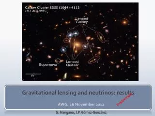
Abell 1689, z=0.183 106 images from 30 sources [Broadhurst et al. 2005]
Free-form mass reconstruction withregularization: Diego et al. (2005b) Cluster Abell 1689 (z=0.183) Errors: rms of many reconstructions using different initial conditions (pixel masses, source positions, source redshifts – within error) Data: 106 images (30 sources) but 601 data pixels Mass pixels: 600, variable size map of S/N ratios 1 arcmin 185 kpc contour lines: reconstructed mass distribution
Mass Modeling Methods Parametric–unknowns:masses, ellipticities, etc. of individual galaxies sufficient for some purposes, but not general enough Kneib et al. (1996), Natarajan et al. (2002), Broadhurst et al. (2004) Free-form – unknowns:usually square pixels tiling the lens plane what to solve for (pixelate potential or mass distribution)? lensing potential – automatically accounts for external shear mass – ensures mass non-negativity what data and errors to use? strong lensing (multiply imaged sources), weak lensing (singly imaged) data with errors: P(D|H,I) is usually a c2-type function data without errors (perfect data): P(D|H,I) replaced by linear constraints how many model parameters (# pixels) to use? comparable to # observables greater than # observables what prior P(H|I) to use? regularization prior (MaxEnt; minimize w.r.t light; smoothing) linear constraints motivated by knowledge of galaxies, clusters how to estimate errors? if regularization – several possibilities if ensemble average: dispersion between individual models AbdelSalam et al. (1997,98), Bradac et al. (2005a,b), Diego et al. (2005a,b) PixeLens: Saha & Williams (2004), Williams & Saha (2005)
Free-form mass reconstruction withensemble averaging: PixeLens Known mass distribution • Solve for mass: • ~30x30 grid of mass pixels • Data: • P(D|H,I) replaced by linear • constraints from image pos. • Priors P(H|I): • mass pixels non-negative • lens center known • density gradient must point within of radial • -0.1 < 2D density slope < -3 • (no smoothness constraint) • Ensemble average: • 200 models, each reproduces • image positions exactly. 5 images (1 source) Blue – true mass contours Black – reconstructed Red – images of point sources 13 images (3 sources)
Free-form mass reconstruction withensemble averaging: PixeLens • Fixed constraints: positions of 4 QSO images • Priors: • external shear PA = 10 45 deg. (Oguri et al. 2004) • -0.25 < 2D density slope < -3.0 • density gradient direction constraint: must point within 45 or 8 deg. from radial SDSS J1004, zQSO =1.734 15’’ 115 kpc blue crosses: galaxies (not used in modeling) red dots: QSO images [Oguri et al. 2004] [Inada et al. 2003, 2005] [Williams & Saha 2005]
Free-form mass reconstruction withensemble averaging: PixeLens SDSS J1004, zQSO =1.734 19 galaxies within 120 kpc of cluster center: comprise <10% of mass, have 3<Mass/Light<15 galaxies were stripped of their DM Mass maps of residuals for 2 PixeLens reconstructions 15’’ 115 kpc blue crosses: galaxies (not used in modeling) red dots: QSO images density slope -1.25 density slope -0.39 [Oguri et al. 2004] [Inada et al. 2003, 2005] [Williams & Saha 2005] contours: …-6.25, -3.15, 0, 3.15, 6.25… x 109MSun/arcsec2 dashed solid
Conclusions Galaxy clusters: In general, mass follows light Galaxies within ~20% of the virial radius are stripped of their DM Unrelaxed clusters: mass peak may not coincide with the cD galaxy Results consistent with the predictions of cold dark matter cosmologies Mass reconstruction methods: Parametric models sufficient for some purposes, but to allow for substructure, galaxies’ variable Mass/Light ratios, misaligned mass/light peaks, and other surprises need more flexible, free-form modeling Open questions in free-form reconstructions: Influence of priors – investigate using reconstructions of synthetic lenses Reducing number of parameters: adaptive pixel size/resolution Principal Components Analysis How to avoid spatially uneven noise distribution in the recovered maps PixeLens – easy to use, open source lens modeling code, with a GUI interface (Saha & Williams 2004); use to find it.