Chapter 6 Electronic Structure of Atoms

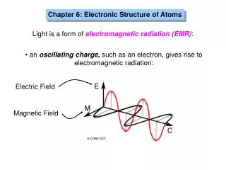
1. Chapter 6Electronic Structure of Atoms David P. White Chapter 6

2. The Wave Nature of Light • All waves have a characteristic wavelength, l, and amplitude, A. • The frequency, f, of a wave is the number of cycles which pass a point in one second. • The speed of a wave, v, is given by its frequency multiplied by its wavelength: • c = fλ • c is the speed of light Chapter 6

3. Chapter 6

5. Modern atomic theory involves interaction of radiation with matter. • Electromagnetic radiation moves through a vacuum with a speed of 3.00  108 m/s. Chapter 6

6. Electromagnetic spectrum

7. Example 1: A laser produces radiation with a wavelength of 640.0 nm. Calculate the frequency of this radiation. Example 2: The YFM radio station broadcasts EM radiation at 99.2 MHz. Calculate the wavelength of this radiation (1 MHz = 106 s-1). Chapter 6

8. Quantized Energy and Photons • Planck: energy can only be absorbed or released from atoms in fixed amounts called quanta. • For 1 photon (energy packet): • E = hf = hc/λ • where h is Planck’s constant (6.63  10-34 J.s). Chapter 6

9. The Photoelectric Effect and Photons • If light shines on the surface of a metal, there is a point (threshold frequency) at which electrons are ejected from the metal. Chapter 6

11. Example 3: (a) A laser emits light with a frequency of 4.69 x 1014s-1. What is the energy of one photon of the radiation from this laser? If the laser emits a pulse of energy containing 5.0 x 1017 photons of this radiation, what is the total energy of that pulse? Chapter 6

12. Line Spectra and the Bohr Model • Line Spectra • Monochromatic light – one λ. • Continuous light – different λs. • White light can be separated into a continuous spectrum of colors. Chapter 6

13. A prism disperses light from a light bulb

14. Balmer: discovered that the lines in the visible line spectrum of hydrogen fit a simple equation. • Later Rydberg generalized Balmer’s equation to: • where RHis the Rydberg constant (1.096776  107 m-1), h is Planck’s constant, n1 and n2 are integers (n2 > n1). Chapter 6

15. Bohr Model explains this equation • Rutherford assumed the electrons orbited the nucleus analogous to planets around the sun. • However, a charged particle moving in a circular path should lose energy, ie, the atom is unstable • Bohr noted the line spectra of certain elements and assumed the electrons were confined to specific energy states called orbits. Chapter 6

16. Colors from excited gases arise because electrons move between energy states in the atom. Black regions show λs absent in the light Chapter 6

17. Bohr Model • Energy states are quantized, light emitted from excited atoms is quantized and appear as line spectra. • Bohr showed that • where n is the principal quantum number (i.e., n = 1, 2, 3). Chapter 6

18. The first orbit has n = 1, is closest to the nucleus, and has negative energy by convention. • The furthest orbit has n close to infinity and corresponds to zero energy. • Electrons in the Bohr model can only move between orbits by absorbing and emitting energy • ∆E = Efinal – Einitial = hf Chapter 6

19. We can show that • When ni > nf, energy is emitted. • When nf > ni, energy is absorbed f Chapter 6

21. Limitations of the Bohr Model • Can only explain the line spectrum of hydrogen adequately. • Electrons are not completely described as small particles. Chapter 6

22. The Wave Behavior of Matter • Explores the wave-like and particle-like nature of matter. • Using Einstein’s and Planck’s equations, de Broglie showed: • The momentum, mv, is a particle property, whereas  is a wave property. Chapter 6

23. The Uncertainty Principle • Heisenberg’s Uncertainty Principle: on the mass scale of atomic particles, we cannot determine exactly the position, direction of motion, and speed simultaneously. • For electrons: we cannot determine their momentum and position simultaneously. • If Dx is the uncertainty in position and Dmv is the uncertainty in momentum, then Chapter 6

24. Quantum Mechanics and Atomic Orbitals • Schrödinger proposed an equation that contains both wave and particle terms. • Solving the equation leads to wave functions, ψ (orbitals). • ψ2 gives the probability of finding the electron • Orbital in the quantum model is different from Bohr’s orbit Chapter 6

25. Chapter 6

26. Schrödinger’s 3 QNs: • Principal Quantum Number, n. - same as Bohr’s n. As n becomes larger, the atom becomes larger and the electron is further from the nucleus. Chapter 6

27. Azimuthal Quantum Number, l. - depends on the value of n. The values of l begin at 0 and increase to (n - 1). The letters for l (s, p, d and f for l = 0, 1, 2, and 3). Usually we refer to the s, p, d and f-orbitals. • Magnetic Quantum Number, ml. - depends on l. Has integral values between -l and +l. Gives the 3D orientation of each orbital. There are (2l +1) allowed values of ml and this gives the no. of orbitals. • Total no. of orbitals in a shell = n2 Chapter 6

28. Chapter 6

29. Orbitals can be ranked in terms of energy to yield an Aufbau diagram. Chapter 6

30. Single electron atom – orbitals with the same value of n have the same energy Chapter 6

31. Representations of Orbitals • The s-Orbitals • All s-orbitals are spherical. • As n increases, the s-orbitals get larger & no. of nodes increase. • A node is a region in space where the probability of finding an electron is zero, 2 = 0. • For an s-orbital, the number of nodes is (n - 1). Chapter 6

33. The p-Orbitals • There are three p-orbitals px, py, and pz. • The letters correspond to allowed values of ml of -1, 0, and +1. • The orbitals are dumbbell shaped and have a node at the nucleus. • As n increases, the p-orbitals get larger. Chapter 6

34. Chapter 6

35. The d and f-Orbitals • There are five d and seven f-orbitals. • They differ in their orientation in the x, y,z plane Chapter 6

37. Many-Electron Atoms • Orbitals and Their Energies • Orbitals of the same energy are said to be degenerate. • For n 2, the s- and p-orbitals are no longer degenerate because the electrons interact with each other. • Therefore, the Aufbau diagram looks different for many-electron systems. Chapter 6

38. Many electron atoms – electrons repel and thus orbitals are at different energies

39. Electron Spin and the Pauli Exclusion Principle • Line spectra of many electron atoms show each line as a closely spaced pair of lines. • Stern and Gerlach designed an experiment to determine why. Chapter 6

40. 2 opposite directions of spin produce oppositely directed magnetic fields leading to the splitting of spectral lines into closely spaced spectra

41. Since electron spin is quantized, we define ms = spin quantum number = + ½ and - ½ . • Pauli’s Exclusion Principle: no two electrons can have the same set of 4 quantum numbers. • Therefore, two electrons in the same orbital must have opposite spins. Chapter 6

42. In the presence of a magnetic field, we can lift the degeneracy of the electrons. Chapter 6

44. Electron Configurations • Hund’s Rule • Electron configurations - in which orbitals the electrons for an element are located. • For degenerate orbitals, electrons fill each orbital singly before any orbital gets a second electron. Chapter 6

45. Condensed Electron Configurations • Neon completes the 2p subshell. • Sodium marks the beginning of a new row. • Na: [Ne] 3s1 • Core electrons: electrons in [Noble Gas]. • Valence electrons: electrons outside of [Noble Gas]. Chapter 6

46. Transition Metals • After Ar the d orbitals begin to fill. • After the 3d orbitals are full, the 4p orbitals begin to fill. • Transition metals: elements in which the d electrons are the valence electrons. Chapter 6

49. Lanthanides and Actinides • From Ce onwards the 4f orbitals begin to fill. • Note: La: [Xe]6s25d14f0 • Elements Ce - Lu have the 4f orbitals filled and are called lanthanides or rare earth elements. • Elements Th - Lr have the 5f orbitals filled and are called actinides. • Most actinides are not found in nature. Chapter 6

50. Electron Configurations and the Periodic Table • The periodic table can be used as a guide for electron configurations. • The period number is the value of n. • Groups 1A and 2A have the s-orbital filled. • Groups 3A - 8A have the p-orbital filled. • Groups 3B - 2B have the d-orbital filled. • The lanthanides and actinides have the f-orbital filled. Chapter 6