Download
1 / 53
530 likes | 572 Vues
Dive into the wave nature of light in Chemistry with a focus on energy quantization, photons, and line spectra according to the 9th Edition of The Central Science. Understand the interaction of radiation with matter and the quantized energy levels of atoms. Explore Planck's constant, the photoelectric effect, and the Bohr model's limitations. Discover the dual nature of matter and light, where wave properties intertwine with particle properties, shaping our understanding of atomic structure.

E N D
CHEMISTRYThe Central Science 9th Edition Chapter 6Electronic Structure of Atoms David P. White Chapter 6
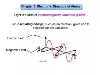
The Wave Nature of Light • All waves have a characteristic wavelength, l, and amplitude, A. • The frequency, n, of a wave is the number of cycles which pass a point in one second. • The speed of a wave, s, is given by its frequency multiplied by its wavelength: • For light, this speed is c. Chapter 6
The Wave Nature of Light Chapter 6
The Wave Nature of Light • Modern atomic theory arose out of studies of the interaction of radiation with matter. • Electromagnetic radiation moves through a vacuum with a speed of 2.99792458 10-8 m/s (3 x 10⁸ m/s). • Electromagnetic waves have characteristic wavelengths and frequencies. • Example: visible radiation has wavelengths between 400 nm (violet) and 750 nm (red). Chapter 6
The Wave Nature of Light Chapter 6
Quantized Energy and Photons • Planck: energy can only be absorbed or released from atoms in certain amounts called quanta. • The relationship between energy and frequency is • where h is Planck’s constant (6.626 10-34 J.s). • To understand quantization consider walking up a ramp versus walking up stairs: • For the ramp, there is a continuous change in height whereas up stairs there is a quantized change in height. Chapter 6
Quantized Energy and Photons • The Photoelectric Effect and Photons • The photoelectric effect provides evidence for the particle nature of light -- “quantization”. • If light shines on the surface of a metal, there is a point at which electrons are ejected from the metal. • The electrons will only be ejected once the threshold frequency is reached. • Below the threshold frequency, no electrons are ejected. • Above the threshold frequency, the number of electrons ejected depend on the intensity of the light. Chapter 6
Quantized Energy and Photons • The Photoelectric Effect and Photons • Einstein assumed that light traveled in energy packets called photons. • The energy of one photon: Chapter 6
Line Spectra and the Bohr Model • Line Spectra • Radiation composed of only one wavelength is called monochromatic. • Radiation that spans a whole array of different wavelengths is called continuous. • White light can be separated into a continuous spectrum of colors. • Note that there are no dark spots on the continuous spectrum that would correspond to different lines. Chapter 6
Line Spectra and the Bohr Model • Line Spectra • Balmer: discovered that the lines in the visible line spectrum of hydrogen fit a simple equation. • Later Rydberg generalized Balmer’s equation to: • where RHis the Rydberg constant (1.096776 107 m-1), h is Planck’s constant (6.626 10-34 J·s), n1 and n2 are integers (n2 > n1). Chapter 6
Line Spectra and the Bohr Model • Bohr Model • Rutherford assumed the electrons orbited the nucleus analogous to planets around the sun. • However, a charged particle moving in a circular path should lose energy. • This means that the atom should be unstable according to Rutherford’s theory. • Bohr noted the line spectra of certain elements and assumed the electrons were confined to specific energy states. These were called orbits. Chapter 6
Line Spectra and the Bohr Model • Bohr Model • Colors from excited gases arise because electrons move between energy states in the atom. Chapter 6
Line Spectra and the Bohr Model • Bohr Model • Since the energy states are quantized, the light emitted from excited atoms must be quantized and appear as line spectra. • After lots of math, Bohr showed that • where n is the principal quantum number (i.e., n = 1, 2, 3, … and nothing else). Chapter 6
Line Spectra and the Bohr Model • Bohr Model • The first orbit in the Bohr model has n = 1, is closest to the nucleus, and has negative energy by convention. • The furthest orbit in the Bohr model has n close to infinity and corresponds to zero energy. • Electrons in the Bohr model can only move between orbits by absorbing and emitting energy in quanta (hn). • The amount of energy absorbed or emitted on movement between states is given by Chapter 6
Line Spectra and the Bohr Model • Bohr Model • We can show that • When ni > nf, energy is emitted. • When nf > ni, energy is absorbed Chapter 6
Line Spectra and the Bohr Model Bohr Model
Line Spectra and the Bohr Model • Limitations of the Bohr Model • Can only explain the line spectrum of hydrogen adequately. • Electrons are not completely described as small particles. Chapter 6
Big Rapis Public Schools: The Wave Behavior of Matter • Knowing that light has a particle nature, it seems reasonable to ask if matter has a wave nature. • Using Einstein’s and Planck’s equations, de Broglie showed: • The momentum, mv, is a particle property, whereas is a wave property. • de Broglie summarized the concepts of waves and particles, with noticeable effects if the objects are small. Chapter 6
The Wave Behavior of Matter • The Uncertainty Principle • Heisenberg’s Uncertainty Principle: on the mass scale of atomic particles, we cannot determine exactly the position, direction of motion, and speed simultaneously. • For electrons: we cannot determine their momentum and position simultaneously. • If Dx is the uncertainty in position and Dmv is the uncertainty in momentum, then Chapter 6
Quantum Mechanics and Atomic Orbitals • Schrödinger proposed an equation that contains both wave and particle terms. • Solving the equation leads to wave functions. • The wave function gives the shape of the electronic orbital. • The square of the wave function, gives the probability of finding the electron, • that is, gives the electron density for the atom. Chapter 6
Quantum Mechanics and Atomic Orbitals Chapter 6
Quantum Mechanics and Atomic Orbitals • Orbitals and Quantum Numbers • If we solve the Schrödinger equation, we get wave functions and energies for the wave functions. • We call wave functions orbitals. • Schrödinger’s equation requires 3 quantum numbers: • Principal Quantum Number, n. This is the same as Bohr’s n. As n becomes larger, the atom becomes larger and the electron is further from the nucleus. Chapter 6
Quantum Mechanics and Atomic Orbitals • Orbitals and Quantum Numbers • Azimuthal Quantum Number, l. This quantum number depends on the value of n. The values of l begin at 0 and increase to (n - 1). We usually use letters for l (s, p, d and f for l = 0, 1, 2, and 3). Usually we refer to the s, p, d and f-orbitals. • Magnetic Quantum Number, ml. This quantum number depends on l. The magnetic quantum number has integral values between -l and +l. Magnetic quantum numbers give the 3D orientation of each orbital. Chapter 6
Quantum Mechanics and Atomic Orbitals • Orbitals and Quantum Numbers Chapter 6
Quantum Mechanics and Atomic Orbitals • Orbitals and Quantum Numbers • Orbitals can be ranked in terms of energy to yield an Aufbau diagram. • Note that the following Aufbau diagram is for a single electron system. • As n increases, note that the spacing between energy levels becomes smaller. Chapter 6
Quantum Mechanics and Atomic Orbitals Orbitals and Quantum Numbers Chapter 6
Quantum Mechanics and Atomic Orbitals • Orbitals and Quantum Numbers Chapter 6
Representations of Orbitals • The s-Orbitals • All s-orbitals are spherical. • As n increases, the s-orbitals get larger. • As n increases, the number of nodes increase. • A node is a region in space where the probability of finding an electron is zero. • At a node, 2 = 0 • For an s-orbital, the number of nodes is (n - 1). Chapter 6
Representations of Orbitals The s-Orbitals Chapter 6
Representations of Orbitals • The p-Orbitals • There are three p-orbitals px, py, and pz. • The three p-orbitals lie along the x-, y- and z- axes of a Cartesian system. • The letters correspond to allowed values of ml of -1, 0, and +1. • The orbitals are dumbbell shaped. • As n increases, the p-orbitals get larger. • All p-orbitals have a node at the nucleus. Chapter 6
Representations of Orbitals The p-Orbitals Chapter 6
Representations of Orbitals • The d and f-Orbitals • There are five d and seven f-orbitals. • Three of the d-orbitals lie in a plane bisecting the x-, y- and z-axes. • Two of the d-orbitals lie in a plane aligned along the x-, y- and z-axes. • Four of the d-orbitals have four lobes each. • One d-orbital has two lobes and a collar. Chapter 6
Many-Electron Atoms • Orbitals and Their Energies • Orbitals of the same energy are said to be degenerate. • For n 2, the s- and p-orbitals are no longer degenerate because the electrons interact with each other. • Therefore, the Aufbau diagram looks slightly different for many-electron systems. Chapter 6
Orbitals and Their Energies Many-Electron Atoms
Many-Electron Atoms • Electron Spin and the Pauli Exclusion Principle • Line spectra of many electron atoms show each line as a closely spaced pair of lines. • Stern and Gerlach designed an experiment to determine why. • A beam of atoms was passed through a slit and into a magnetic field and the atoms were then detected. • Two spots were found: one with the electrons spinning in one direction and one with the electrons spinning in the opposite direction. Chapter 6
Many-Electron Atoms Electron Spin and the Pauli Exclusion Principle
Many-Electron Atoms • Electron Spin and the Pauli Exclusion Principle • Since electron spin is quantized, we define ms = spin quantum number = ½. • Pauli’s Exclusions Principle: no two electrons can have the same set of 4 quantum numbers. • Therefore, two electrons in the same orbital must have opposite spins. Chapter 6
Many-Electron Atoms • Electron Spin and the Pauli Exclusion Principle • In the presence of a magnetic field, we can lift the degeneracy of the electrons. Chapter 6
Electron Configurations • Hund’s Rule • Electron configurations tells us in which orbitals the electrons for an element are located. • Three rules: • electrons fill orbitals starting with lowest n and moving upwards; • no two electrons can fill one orbital with the same spin (Pauli); • for degenerate orbitals, electrons fill each orbital singly before any orbital gets a second electron (Hund’s rule). Chapter 6
Electron Configurations • Condensed Electron Configurations • Neon completes the 2p subshell. • Sodium marks the beginning of a new row. • So, we write the condensed electron configuration for sodium as • Na: [Ne] 3s1 • [Ne] represents the electron configuration of neon. • Core electrons: electrons in [Noble Gas]. • Valence electrons: electrons outside of [Noble Gas]. Chapter 6
Electron Configurations • Transition Metals • After Ar the d orbitals begin to fill. • After the 3d orbitals are full, the 4p orbitals being to fill. • Transition metals: elements in which the d electrons are the valence electrons. Chapter 6
Electron Configurations • Lanthanides and Actinides • From Ce onwards the 4f orbitals begin to fill. • Note: La: [Xe]6s25d14f0 • Elements Ce - Lu have the 4f orbitals filled and are called lanthanides or rare earth elements. • Elements Th - Lr have the 5f orbitals filled and are called actinides. • Most actinides are not found in nature. Chapter 6
Electron Configurations and the Periodic Table • The periodic table can be used as a guide for electron configurations. • The period number is the value of n. • Groups 1A and 2A have the s-orbital filled. • Groups 3A - 8A have the p-orbital filled. • Groups 3B - 2B have the d-orbital filled. • The lanthanides and actinides have the f-orbital filled. Chapter 6