Chapter 6 Electronic Structure of Atoms
410 likes | 679 Vues
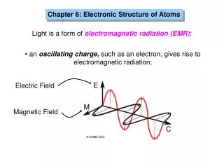
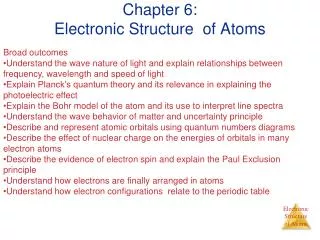
Chemistry, The Central Science , 11th edition Theodore L. Brown; H. Eugene LeMay, Jr.; and Bruce E. Bursten. Chapter 6 Electronic Structure of Atoms. John D. Bookstaver St. Charles Community College Cottleville, MO. Waves.

Chapter 6 Electronic Structure of Atoms
E N D
Presentation Transcript
Chemistry, The Central Science, 11th edition Theodore L. Brown; H. Eugene LeMay, Jr.; and Bruce E. Bursten Chapter 6Electronic Structureof Atoms John D. Bookstaver St. Charles Community College Cottleville, MO © 2009, Prentice-Hall, Inc.
Waves • To understand the electronic structure of atoms, one must understand the nature of electromagnetic radiation. • The distance between corresponding points on adjacent waves is the wavelength (). © 2009, Prentice-Hall, Inc.
Waves • The number of waves passing a given point per unit of time is the frequency(). • For waves traveling at the same velocity, the longer the wavelength, the smaller the frequency. © 2009, Prentice-Hall, Inc.
Electromagnetic Radiation • All electromagnetic radiation travels at the same velocity: the speed of light (c), 3.00 108 m/s. • Therefore, c = © 2009, Prentice-Hall, Inc.
The Nature of Energy • The wave nature of light does not explain how an object can glow when its temperature increases. • Max Planck explained it by assuming that energy comes in packets called quanta. © 2009, Prentice-Hall, Inc.
The Nature of Energy • Einstein used this assumption to explain the photoelectric effect. • He concluded that energy is proportional to frequency: E = h where h is Planck’s constant, 6.626 10−34 J-s. © 2009, Prentice-Hall, Inc.
The Nature of Energy • Therefore, if one knows the wavelength of light, one can calculate the energy in one photon, or packet, of that light: c = E = h © 2009, Prentice-Hall, Inc.
The Nature of Energy Another mystery in the early 20th century involved the emission spectra observed from energy emitted by atoms and molecules. © 2009, Prentice-Hall, Inc.
The Nature of Energy • For atoms and molecules one does not observe a continuous spectrum, as one gets from a white light source. • Only a line spectrum of discrete wavelengths is observed. © 2009, Prentice-Hall, Inc.
The Nature of Energy • Niels Bohr adopted Planck’s assumption and explained these phenomena in this way: • Electrons in an atom can only occupy certain orbits (corresponding to certain energies). © 2009, Prentice-Hall, Inc.
The Nature of Energy • Niels Bohr adopted Planck’s assumption and explained these phenomena in this way: • Electrons in permitted orbits have specific, “allowed” energies; these energies will not be radiated from the atom. © 2009, Prentice-Hall, Inc.
The Nature of Energy • Niels Bohr adopted Planck’s assumption and explained these phenomena in this way: • Energy is only absorbed or emitted in such a way as to move an electron from one “allowed” energy state to another; the energy is defined by E = h © 2009, Prentice-Hall, Inc.
1 nf2 ( ) - E = −RH 1 ni2 The Nature of Energy The energy absorbed or emitted from the process of electron promotion or demotion can be calculated by the equation: where RH is the Rydberg constant, 2.18 10−18 J, and ni and nf are the initial and final energy levels of the electron. © 2009, Prentice-Hall, Inc.
h mv = The Wave Nature of Matter • Louis de Broglie posited that if light can have material properties, matter should exhibit wave properties. • He demonstrated that the relationship between mass and wavelength was © 2009, Prentice-Hall, Inc.
h 4 (x) (mv) The Uncertainty Principle • Heisenberg showed that the more precisely the momentum of a particle is known, the less precisely is its position known: • In many cases, our uncertainty of the whereabouts of an electron is greater than the size of the atom itself! © 2009, Prentice-Hall, Inc.
Quantum Mechanics • Erwin Schrödinger developed a mathematical treatment into which both the wave and particle nature of matter could be incorporated. • It is known as quantum mechanics. © 2009, Prentice-Hall, Inc.
Quantum Mechanics • The wave equation is designated with a lower case Greek psi (). • The square of the wave equation, 2, gives a probability density map of where an electron has a certain statistical likelihood of being at any given instant in time. © 2009, Prentice-Hall, Inc.
Quantum Numbers • Solving the wave equation gives a set of wave functions, or orbitals, and their corresponding energies. • Each orbital describes a spatial distribution of electron density. • An orbital is described by a set of three quantum numbers. © 2009, Prentice-Hall, Inc.
Principal Quantum Number (n) • The principal quantum number, n, describes the energy level on which the orbital resides. • The values of n are integers ≥ 1. © 2009, Prentice-Hall, Inc.
Angular Momentum Quantum Number (l) • This quantum number defines the shape of the orbital. • Allowed values of l are integers ranging from 0 to n −1. • We use letter designations to communicate the different values of l and, therefore, the shapes and types of orbitals. © 2009, Prentice-Hall, Inc.
Angular Momentum Quantum Number (l) © 2009, Prentice-Hall, Inc.
Magnetic Quantum Number (ml) • The magnetic quantum number describes the three-dimensional orientation of the orbital. • Allowed values of ml are integers ranging from -l to l: −l ≤ ml≤ l. • Therefore, on any given energy level, there can be up to 1 s orbital, 3 p orbitals, 5 d orbitals, 7 f orbitals, etc. © 2009, Prentice-Hall, Inc.
Magnetic Quantum Number (ml) • Orbitals with the same value of n form a shell. • Different orbital types within a shell are subshells. © 2009, Prentice-Hall, Inc.
s Orbitals • The value of l for s orbitals is 0. • They are spherical in shape. • The radius of the sphere increases with the value of n. © 2009, Prentice-Hall, Inc.
s Orbitals Observing a graph of probabilities of finding an electron versus distance from the nucleus, we see that s orbitals possess n−1 nodes, or regions where there is 0 probability of finding an electron. © 2009, Prentice-Hall, Inc.
p Orbitals • The value of l for p orbitals is 1. • They have two lobes with a node between them. © 2009, Prentice-Hall, Inc.
d Orbitals • The value of l for a d orbital is 2. • Four of the five d orbitals have 4 lobes; the other resembles a p orbital with a doughnut around the center. © 2009, Prentice-Hall, Inc.
Energies of Orbitals • For a one-electron hydrogen atom, orbitals on the same energy level have the same energy. • That is, they are degenerate. © 2009, Prentice-Hall, Inc.
Energies of Orbitals • As the number of electrons increases, though, so does the repulsion between them. • Therefore, in many-electron atoms, orbitals on the same energy level are no longer degenerate. © 2009, Prentice-Hall, Inc.
Spin Quantum Number, ms • In the 1920s, it was discovered that two electrons in the same orbital do not have exactly the same energy. • The “spin” of an electron describes its magnetic field, which affects its energy. © 2009, Prentice-Hall, Inc.
Spin Quantum Number, ms • This led to a fourth quantum number, the spin quantum number, ms. • The spin quantum number has only 2 allowed values: +1/2 and −1/2. © 2009, Prentice-Hall, Inc.
Pauli Exclusion Principle • No two electrons in the same atom can have exactly the same energy. • Therefore, no two electrons in the same atom can have identical sets of quantum numbers. © 2009, Prentice-Hall, Inc.
Electron Configurations • This shows the distribution of all electrons in an atom. • Each component consists of • A number denoting the energy level, © 2009, Prentice-Hall, Inc.
Electron Configurations • This shows the distribution of all electrons in an atom • Each component consists of • A number denoting the energy level, • A letter denoting the type of orbital, © 2009, Prentice-Hall, Inc.
Electron Configurations • This shows the distribution of all electrons in an atom. • Each component consists of • A number denoting the energy level, • A letter denoting the type of orbital, • A superscript denoting the number of electrons in those orbitals. © 2009, Prentice-Hall, Inc.
Orbital Diagrams • Each box in the diagram represents one orbital. • Half-arrows represent the electrons. • The direction of the arrow represents the relative spin of the electron. © 2009, Prentice-Hall, Inc.
Hund’s Rule “For degenerate orbitals, the lowest energy is attained when the number of electrons with the same spin is maximized.” © 2009, Prentice-Hall, Inc.
Periodic Table • We fill orbitals in increasing order of energy. • Different blocks on the periodic table (shaded in different colors in this chart) correspond to different types of orbitals. © 2009, Prentice-Hall, Inc.
Some Anomalies Some irregularities occur when there are enough electrons to half-fill s and d orbitals on a given row. © 2009, Prentice-Hall, Inc.
Some Anomalies For instance, the electron configuration for copper is [Ar] 4s1 3d5 rather than the expected [Ar] 4s2 3d4. © 2009, Prentice-Hall, Inc.
Some Anomalies • This occurs because the 4s and 3d orbitals are very close in energy. • These anomalies occur in f-block atoms, as well. © 2009, Prentice-Hall, Inc.