DACIDR: Clustering & Dimension Reduction Method
220 likes | 322 Vues
Innovative method for solving taxonomy-independent analysis problems, tackling millions of data accurately. Features pairwise clustering, multidimensional scaling, interpolation, and visualization. Utilizes DACIDR flow chart for streamlined analysis process.

DACIDR: Clustering & Dimension Reduction Method
E N D
Presentation Transcript
DACIDRA Deterministic Annealing Clustering and Interpolative Dimension Reduction Method Yang Ruan PhD Candidate Salsahpc Group Community Grid Lab Indiana University
Overview • Solve Taxonomy independent analysis problem for millions of datawith a high accuracy solution. • Introduction to DACIDR • All-pair sequence alignment • Pairwise Clustering and Multidimensional Scaling • Interpolation • Visualization • SSP-Tree • Experiments
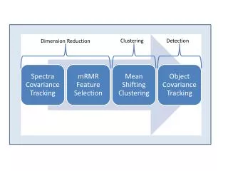
DACIDR Flow Chart 16S rRNA Data Sample Set Out-sample Set Pairwise Clustering All-Pair Sequence Alignment Sample Clustering Result Dissimilarity Matrix Multidimensional Scaling Heuristic Interpolation Target Dimension Result Further Analysis Visualization
All-Pair Sequence Analysis • Input: FASTA File • Output: Dissimilarity Matrix • Use Smith Waterman alignment to perform local sequence alignment to determine similar regions between two nucleotide or protein sequences. • Use percentage identity as similarity measurement. - =17 ACATCCTTAACAA - - ATTGC-ATC - AGT - CTA = 0.47 =32 ACATCCTTAGC - - GAATT - - TATGAT - CACCA
DACIDR Flow Chart 16S rRNA Data Sample Set Out-sample Set Pairwise Clustering All-Pair Sequence Alignment Sample Clustering Result Dissimilarity Matrix Multidimensional Scaling Heuristic Interpolation Target Dimension Result Further Analysis Visualization
DA Pairwise Clustering • Input: Dissimilarity Matrix • Output: Clustering result • Deterministic Annealing clustering is a robust clustering method. • Temperature corresponds to pairwise distance scale and one starts at high temperature with all sequences in same cluster. As temperature is lowered one looks at finer distance scale and additional clusters are automatically detected. • No heuristic input is needed.
Multidimensional Scaling • Input: Dissimilarity Matrix • Output: Visualization Result (in 3D) • MDS is a set of techniques used in dimension reduction. • Scaling by Majorizing a Complicated Function (SMACOF) is a fast EM method for distributed computing. • DA introduce temperature into SMACOF which can eliminates the local optima problem.
DACIDR Flow Chart 16S rRNA Data Sample Set Out-sample Set Pairwise Clustering All-Pair Sequence Alignment Sample Clustering Result Dissimilarity Matrix Multidimensional Scaling Heuristic Interpolation Target Dimension Result Further Analysis Visualization
Interpolation • Input: Sample Set Result/Out-sample Set FASTA File • Output: Full Set Result. • SMACOF uses O(N2) memory, which could be a limitation for million-scale dataset • MI-MDS finds k nearest neighbor (k-NN) points in the sample set for sequences in the out-sample set. Then use this k points to determine the out-sample dimension reduction result. • It doesn’t need O(N2) memory and can be pleasingly parallelized.
DACIDR Flow Chart 16S rRNA Data Sample Set Out-sample Set Pairwise Clustering All-Pair Sequence Alignment Sample Clustering Result Dissimilarity Matrix Multidimensional Scaling Heuristic Interpolation Target Dimension Result Further Analysis Visualization
Visualization • Used PlotViz3 to visualize the 3D plot generated in previous step. • It can show the sequence name, highlight interesting points, even remotely connect to HPC cluster and do dimension reduction and streaming back result. Rotate Zoom in
SSP-Tree • Sample Sequence Partition Tree is a method inspired by Barnes-Hut Tree used in astrophysics simulations. • SSP-Tree is an octree to partition the sample sequence space in 3D. i0 i1 e4 i2 e5 F E e0 e2 e1 e3 e6 e7 A B C D G H a An example for SSP-Tree in 2D with 8 points
Heuristic Interpolation • MI-MDS has to compare every out-sample point to every sample point to find k-NN points • HI-MDS compare with each center point of each tree node, and searches k-NN points from top to bottom • HE-MDS directly search nearest terminal node and find k-NN points within that node or its nearest nodes. • Computation complexity • MI-MDS: O(NM) • HI-MDS: O(NlogM) • HE-MDS: O(N(NT + MT)) 3D plot after HE-MI
Region Refinement Before • Terminal nodes can be divided into: • V: Inter-galactic void • U: Undecided node • G: Decided node • Take H(t) to determine if a terminal node t should be assigned to V • Take a fraction function F(t) to determine if a terminal node t should be assigned to G. • Update center points of each terminal node t at the end of each iteration. After
Recursive Clustering • DACIDR create an initial clustering result W = {w1, w2, w3, … wr}. • Possible Interesting Structures inside each mega region. • w1 -> W1’ = {w11’, w12’, w13’, …, w1r1’}; • w2-> W2’ = {w21’, w22’, w23’, …, w2r2’}; • w3-> W3’ = {w31’, w32’, w33’, …, w3r3’}; • … • wr-> Wr’ = {wr1’, wr2’, wr3’, …, wrrr’}; Mega Region 1 Recursive Clustering
Experiments • Clustering and Visualization • Input Data: 1.1 million 16S rRNA data • Environment: 32 nodes (768 cores) of Tempest and 100 nodes (800 cores) of PolarGrid. • SW vs NW • PWC vs UCLUST/CDHIT • HE-MI vs MI-MDS/HI-MI
SW vs NW SW • Smith Waterman performs local alignment while Needleman Wunsch performs global alignment. • Global alignment suffers problem from various lengths in this dataset NW
PWC vs UCLUST/CDHIT PWC • PWC shows much more robust result than UCLUST and CDHIT • PWC has a high correlation with visualized clusters while UCLUST/CDHIT shows a worse result UCLUST
HE-MI vs MI-MDS/HI-MI • Input set: 100k subset from 1.1 million data • Environment: 32 nodes (256 cores) from PolarGrid • Compared time and normalized stress value:
Conclusion • By using SSP-Tree inside DACIDR, we sucessfully clustered and visualized 1.1 million 16S rRNA data • Distance measurement is important in clustering and visualization as SW and NW will give quite different answers when sequence lengths varies. • DA-PWC performs much better than UCLUST/CDHIT • HE-MI has a slight higher stress value than MI-MDS, but is almost 100 times faster than the latter one, which makes it suitable for massive scale dataset.
Futurework • We are experimenting using different techniques choosing reference set from the clustering result we have. • To do further study about the taxonomy-independent clustering result we have, phylogenetic tree are generated with some sequences selected from known samples. • Visualized phylogenetic tree in 3D to help biologist better understand it.