Deterministic Annealing

1. Deterministic Annealing Geoffrey Fox gcf@indiana.edu http://www.infomall.orghttp://www.futuregrid.org Director, Digital Science Center, Pervasive Technology Institute Associate Dean for Research and Graduate Studies,  School of Informatics and Computing Indiana University Bloomington Indiana University CS Theory group January 23 2012

2. Abstract • We discuss general theory behind deterministic annealing and illustrate with applications to mixture models (including GTM and PLSA), clustering and dimension reduction. • We cover cases where the analyzed space has a metric and cases where it does not. • We discuss the many open issues and possible further work for methods that appear to outperform the standard approaches but are in practice not used.

3. References • Ken Rose, Deterministic Annealing for Clustering, Compression, Classification, Regression, and Related Optimization Problems. Proceedings of the IEEE, 1998. 86: p. 2210--2239. • References earlier papers including his Caltech Elec. Eng. PhD 1990 • T Hofmann, JM Buhmann, “Pairwise data clustering by deterministic annealing”, IEEE Transactions on Pattern Analysis and Machine Intelligence 19, pp1-13 1997. • HansjörgKlock and Joachim M. Buhmann, “Data visualization by multidimensional scaling: a deterministic annealing approach”, Pattern Recognition, Volume 33, Issue 4, April 2000, Pages 651-669. • FrühwirthR, Waltenberger W: Redescending M-estimators and Deterministic Annealing, with Applications to Robust Regression and Tail Index Estimation. http://www.stat.tugraz.at/AJS/ausg083+4/08306Fruehwirth.pdf   Austrian Journal of Statistics 2008, 37(3&4):301-317. • Review http://grids.ucs.indiana.edu/ptliupages/publications/pdac24g-fox.pdf • Recent algorithm work by Seung-Hee Bae, Jong YoulChoi (Indiana CS PhD’s) • http://grids.ucs.indiana.edu/ptliupages/publications/CetraroWriteupJune11-09.pdf • http://grids.ucs.indiana.edu/ptliupages/publications/hpdc2010_submission_57.pdf

4. Some Goals • We are building a library of parallel data mining tools that have best known (to me) robustness and performance characteristics • Big data needs super algorithms? • A lot of statistics tools (e.g. in R) are not the best algorithm and not always well parallelized • Deterministic annealing (DA) is one of better approaches to optimization • Tends to remove local optima • Addresses overfitting • Faster than simulated annealing • Return to my heritage (physics) with an approach I called Physical Computation (cf. also genetic algs) -- methods based on analogies to nature • Physics systems find true lowest energy state if you anneal i.e. you equilibrate at each temperature as you cool

5. Some Ideas I • Deterministic annealing is better than many well-used optimization problems • Started as “Elastic Net” by Durbin for Travelling Salesman Problem TSP • Basic idea behind deterministic annealing is mean field approximation, which is also used in “Variational Bayes” and many “neural network approaches” • Markov chain Monte Carlo (MCMC) methods are roughly single temperature simulated annealing • Less sensitive to initial conditions • Avoid local optima • Not equivalent to trying random initial starts

6. Some non-DA Ideas II • Dimension reduction gives Low dimension mappings of data to both visualize and apply geometric hashing • No-vector (can’t define metric space) problems are O(N2) • For no-vector case, one can develop O(N) or O(NlogN) methods as in “Fast Multipole and OctTree methods” • Map high dimensional data to 3D and use classic methods developed originally to speed up O(N2) 3D particle dynamics problems

7. Uses of Deterministic Annealing • Clustering • Vectors: Rose (Gurewitz and Fox) • Clusters with fixed sizes and no tails (Proteomics team at Broad) • No Vectors: Hofmann and Buhmann (Just use pairwise distances) • Dimension Reduction for visualization and analysis • Vectors: GTM • No vectors: MDS (Just use pairwise distances) • Can apply to general mixture models (but less study) • Gaussian Mixture Models • Probabilistic Latent Semantic Analysis with Deterministic Annealing DA-PLSA as alternative to Latent Dirichlet Allocation (typical informational retrieval/global inference topic model)

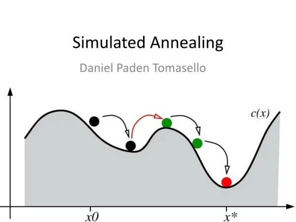
8. Deterministic Annealing I • Gibbs Distribution at Temperature TP() = exp( - H()/T) /  d exp( - H()/T) • Or P() = exp( - H()/T + F/T ) • Minimize Free Energy combining Objective Function and EntropyF= < H- T S(P) > =  d {P()H+ T P() lnP()} • Where  are (a subset of) parameters to be minimized • Simulated annealing corresponds to doing these integrals by Monte Carlo • Deterministic annealing corresponds to doing integrals analytically (by mean field approximation) and is naturally much faster than Monte Carlo • In each case temperature is lowered slowly – say by a factor 0.95 to 0.99 at each iteration

9. DeterministicAnnealing • Minimum evolving as temperature decreases • Movement at fixed temperature going to local minima if not initialized “correctly F({y}, T) Solve Linear Equations for each temperature Nonlinear effects mitigated by initializing with solution at previous higher temperature Configuration {y}

10. Deterministic Annealing II Note 3 types of variablesused to approximate real Hamiltonian subject to annealing The rest – optimized by traditional methods • For some cases such as vector clustering and Mixture Models one can do integrals by hand but usually will be impossible • So introduce Hamiltonian H0(, ) which by choice of can be made similar to real Hamiltonian HR() and which has tractable integrals • P0() = exp( - H0()/T + F0/T ) approximate Gibbs for HR • FR (P0) = < HR - T S0(P0) >|0 = < HR – H0> |0 + F0(P0) • Where <…>|0 denotes  d Po() • Easy to show that real Free Energy (the Gibb’s inequality)FR (PR) ≤ FR (P0) (Kullback-Leibler divergence) • Expectation step E is find  minimizing FR (P0) and • Follow with M step (of EM) setting  = <> |0 =  dPo() (mean field) and one follows with a traditional minimization of remaining parameters

11. Implementation of DA Central Clustering • Clustering variables are Mi(k) (these are annealed  in general approach) where this is probability point ibelongs to cluster k andk=1KMi(k) = 1 • In Central or PW Clustering, take H0 = i=1Nk=1K Mi(k) i(k) • Linear form allows DA integrals to be done analytically • Central clustering hasi(k) = (X(i)- Y(k))2 and Mi(k) determined by Expectation step • HCentral = i=1Nk=1KMi(k) (X(i)- Y(k))2 • Hcentraland H0are identical • <Mi(k)> = exp( -i(k)/T ) / k=1Kexp( -i(k)/T ) • Centers Y(k) are determined in M step

12. Implementation of DA-PWC • Clustering variables are again Mi(k) (these are  in general approach) where this is probability point ibelongs to cluster k • Pairwise Clustering Hamiltonian given by nonlinear form • HPWC= 0.5 i=1Nj=1N(i, j) k=1KMi(k) Mj(k) / C(k) • (i, j) is pairwise distance between points i and j • with C(k) = i=1NMi(k) as number of points in Cluster k • Take same form H0 = i=1Nk=1K Mi(k) i(k) as for central clustering • i(k) determined to minimize FPWC (P0) = < HPWC - T S0(P0) >|0where integrals can be easily done • And now linear (in Mi(k)) H0 and quadratic HPC are different • Again <Mi(k)> = exp( -i(k)/T ) / k=1Kexp( -i(k)/T )

13. General Features of DA • Deterministic Annealing DA is related to Variational Inference or Variational Bayes methods • In many problems, decreasing temperature is classic multiscale – finer resolution (√T is “just” distance scale) • We have factors like (X(i)- Y(k))2/ T • In clustering, one then looks at second derivative matrix of FR (P0) wrtand as temperature is lowered this develops negative eigenvalue corresponding to instability • Or have multiple clusters at each center and perturb • This is a phase transition and one splits cluster into two and continues EM iteration • One can start with just one cluster

14. Rose, K., Gurewitz, E., and Fox, G. C. ``Statistical mechanics and phase transitions in clustering,'' Physical Review Letters, 65(8):945-948, August 1990. My #6 most cited article (402 citesincluding 15 in 2011)

15. Start at T= “” with 1 Cluster • Decrease T, Clusters emerge at instabilities

18. DA-PWC EM Steps (E is red, M Black)k runs over clusters; i,j points • A(k) = - 0.5 i=1Nj=1N(i, j) <Mi(k)> <Mj(k)> / <C(k)>2 • Bi(k) = j=1N(i, j) <Mj(k)> / <C(k)> • i(k) = (Bi(k) + A(k)) • <Mi(k)> = exp( -i(k)/T )/k=1Kexp(-i(k)/T) • C(k) = i=1N<Mi(k)> • Loop to converge variables; decrease T from  i points k clusters Parallelize by distributing points across processes Steps 1 global sum (reduction) Step 1, 2, 5 local sum if <Mi(k)> broadcast

19. Continuous Clustering I • This is a subtlety introduced by Ken Rose but not clearly known in community • Lets consider “dynamic appearance” of clusters a little more carefully. We suppose that we take a cluster k and split into 2 with centers Y(k)A and Y(k)B with initial valuesY(k)A = Y(k)B at original center Y(k) • Then typically if you make this change and perturb the Y(k)AY(k)B, they will return to starting position as F at stable minimum • But instability can develop and one finds Free Energy F Y(k)A and Y(k)B Free Energy F Free Energy F Y(k)A- Y(k)B Y(k)A+ Y(k)B

20. Continuous Clustering II • At phase transition when eigenvalue corresponding to Y(k)A - Y(k)B goes negative, F is a minimum if two split clusters move together but a maximum if they separate • i.e. two genuine clusters are formed at instability points • When you split A(k) , Bi(k), i(k) are unchanged and you would hope that cluster counts C(k) and probabilities <Mi(k)> would be halved • Unfortunately that doesn’t work except for 1 cluster splitting into 2 due to factor Zi = k=1Kexp(-i(k)/T) with <Mi(k)> = exp( -i(k)/T )/Zi • Naïve solution is to examine explicitly solution with A(k0) , Bi(k0), i(k0) are unchanged; C(k0), <Mi(k0)> halved for 0 <= k0 < K andZi = k=1Kw(k)exp(-i(k)/T) with w(k0) =2, w(kk0) = 1 • Works surprisingly well but much more elegant is Continuous Clustering

21. Continuous Clustering III • You restate problem to consider from the start an arbitrary number of cluster centers at each center with • p(k) the density of clusters at site k • All these clusters at a given site have same parameters • Zi = k=1Kp(k) exp(-i(k)/T) with <Mi(k)> = p(k) exp( -i(k)/T )/Zi and k=1K p(k) = 1 • You can then consider p(k) as one of the non-annealed parameters (the centers Y(k) in central clustering were of this type) determined in final M step. This gives p(k) = C(k) / N • Which interestingly weights clusters according to their size giving all points “equal weight” • Initial investigation says similar in performance to naïve case • Now splitting is exact. p(k), C(k) and probabilities <Mi(k)> are halved. A(k) , Bi(k), i(k) are unchanged

22. DA-PWC EM Steps (E is red, M Black)k runs over clusters; i,j points • A(k) = - 0.5 i=1Nj=1N(i, j) <Mi(k)> <Mj(k)> / <C(k)>2 • Bj(k) = i=1N(i, j) <Mi(k)> / <C(k)> • i(k) = (Bi(k) + A(k)) • <Mi(k)> = p(k) exp( -i(k)/T )/k=1K p(k) exp(-i(k)/T) • C(k) = i=1N<Mi(k)> • p(k) = C(k) / N • Loop to converge variables; decrease T from ; split centers by halving p(k) Steps 1 global sum (reduction) Step 1, 2, 5 local sum if <Mi(k)> broadcast

23. Note on Performance • Algorithms parallelize well with typical speed up of 500 on 768 cores • Parallelization is very straightforward • The calculation of eigenvectors of second derivative matrix on pairwise case is ~80% effort • Need to use power method to find leading eigenvectors for each cluster • Eigenvector is of length N (number of points) for pairwise • In central clustering, eigenvector of length “dimension of space” • To do: Compare calculation of eigenvectors with splitting and perturbing each cluster center and see if stable • Note eigenvector method tells you direction of instability

24. Trimmed Clustering • Clustering with position-specific constraints on variance: Applying redescending M-estimators to label-free LC-MS data analysis (Rudolf Frühwirth, D R Mani and SaumyadiptaPyne) BMC Bioinformatics 2011, 12:358 • HTCC= k=0Ki=1NMi(k) f(i,k) • f(i,k) = (X(i) - Y(k))2/2(k)2 k > 0 • f(i,0) = c2 / 2 k = 0 • The 0’th cluster captures (at zero temperature) all points outside clusters (background) • Clusters are trimmed (X(i) - Y(k))2/2(k)2< c2 / 2 • Another case when H0 is same as target Hamiltonian • Proteomics Mass Spectrometry T = 1 T ~ 0 T = 5 Distance from cluster center

25. High Performance Dimension Reduction and Visualization • Need is pervasive • Large and high dimensional data are everywhere: biology, physics, Internet, … • Visualization can help data analysis • Visualization of large datasets with high performance • Map high-dimensional data into low dimensions (2D or 3D). • Need Parallel programming for processing large data sets • Developing high performance dimension reduction algorithms: • MDS(Multi-dimensional Scaling) • GTM(Generative Topographic Mapping) • DA-MDS(Deterministic Annealing MDS) • DA-GTM(Deterministic Annealing GTM) • Interactive visualization tool PlotViz

26. Multidimensional Scaling MDS • Map points in high dimension to lower dimensions • Many such dimensionreductionalgorithms (PCA Principal component analysis easiest); simplest but perhaps best at times is MDS • Minimize Stress (X) = i<j=1nweight(i,j) ((i, j) - d(Xi , Xj))2 • (i, j) are input dissimilarities and d(Xi , Xj) the Euclidean distance squared in embedding space (3D usually) • SMACOF or Scaling by minimizing a complicated function is clever steepest descent (expectation maximization EM) algorithm • Computational complexity goes like N2* Reduced Dimension • We describe Deterministic annealed version of it which is much better • Could just view as non linear 2problem (Tapia et al. Rice) • Slower but more general • All parallelize with high efficiency

27. Implementation of MDS • HMDS = i< j=1nweight(i,j) ((i, j) - d(X(i) , X(j)))2 • Where (i, j) are observed dissimilarities and we want to represent as Euclidean distance d between points X(i) and X(j) • HMDS is quartic or involves square roots, so we need the idea of an approximate Hamiltonian H0 • One tractable integral form for H0 was linear Hamiltonians • Another is Gaussian H0 = i=1n (X(i)- (i))2 / 2 • Where X(i)are vectors to be determined as in formula for Multidimensional scaling • The E step is minimize i< j=1nweight(i,j) ((i, j) – constant.T - ((i) - (j))2 )2 • with solution (i) = 0 at large Temperature T • Points pop out from origin as Temperature lowered

28. Pairwise Clustering and MDS are O(N2) Problems • 100,000 sequences takes a few days on 768 cores 32 nodes Windows Cluster Tempest • Could just run 680K on 6.82 larger machine but lets try to be “cleverer” and use hierarchical methods • Start with 100K sample run fully • Divide into “megaregions” using 3D projection • Interpolate full sample into megaregions and analyze latter separately • See http://salsahpc.org/millionseq/16SrRNA_index.html

29. Use Barnes Hut OctTree originally developed to make O(N2) astrophysics O(NlogN)

30. OctTree for 100K sample of Fungi We use OctTree for logarithmic interpolation

31. 440K Interpolated

32. A large cluster in Region 0

33. 26 Clusters in Region 4

34. 13 Clusters in Region 6

35. Quality of DA versus EM MDS Normalized STRESS Variation in different runs Map to 2D 100K Metagenomics Map to 3D

36. Run Time of DA versus EM MDS Run time secs Map to 2D 100K Metagenomics Map to 3D

37. GTM with DA (DA-GTM) • GTM is an algorithm for dimension reduction • Find optimal K latent variables in Latent Space • f is a non-linear mapping function • Traditional algorithm use EM for model fitting • DA optimization can improve the fitting process Map to Grid (like SOM) K latent points N data points

38. Advantages of GTM • Computational complexity is O(KN), where • N is the number of data points • K is the number of latent variables or clusters. K << N • Efficient, compared with MDS which is O(N2) • Produce more separable map (right) than PCA (left) GTM PCA Oil flow data 1000 points 12 Dimensions 3 Clusters

39. Free Energy for DA-GTM • Free Energy • D : expected distortion • H : Shannon entropy • T : computational temperature • Zn : partitioning function • Partition Function for GTM

40. DA-GTM vs. EM-GTM EM-GTM DA-GTM Optimization Maximize log-likelihood L Minimize free energy F ObjectiveFunction When T = 1, L = -F. Pros & Cons • Very sensitive • Trapped in local optima • Faster • Large deviation • Less sensitive to an initial condition • Find global optimum • Require more computational time • Smaller standard deviation

41. DA-GTM Result 496 466 427 511 (α = 0.95) (α = 0.99) (1stTc = 4.64)

42. Data Mining Projects using GTM Visualizing 215 solvents by GTM-Interpolation 215 solvents (colored and labeled) are embedded with 100,000 chemical compounds (colored in grey) in PubChem database Chemical compounds reported in literatures Visualized 234,000 chemical compounds which may be related with a set of 5 genes of interest (ABCB1, CHRNB2, DRD2, ESR1, and F2) based on the dataset collected from major journal literatures PubChem data with CTD visualization About 930,000 chemical compounds are visualized in a 3D space, annotated by the related genes in Comparative Toxicogenomics Database (CTD)

43. Probabilistic Latent Semantic Analysis (PLSA) • Topic model (or latent model) • Assume generative K topics (document generator) • Each document is a mixture of K topics • The original proposal used EM for model fitting Topic 1 Topic 2 Topic K Doc 1 Doc 2 Doc N

44. DA-Mixture Models • Mixture models take general formH = - n=1N k=1KMn(k) ln L(n|k)k=1KMn(k) = 1 for each nn runs over things being decomposed (documents in this case)k runs over component things– Grid points for GTM, Gaussians for Gaussian mixtures, topics for PLSA • Anneal on “spins” Mn(k) so H is linear and do not need another Hamiltonian as H = H0 • Note L(n|k) is function of “interesting” parameters and these are found as in non annealed case by a separate optimization in the M step

45. EM vs. DA-{GTM, PLSA} EM DA Optimization Maximize log-likelihood L Minimize free energy F ObjectiveFunctions GTM PLSA Note: When T = 1, L = -F. This implies EM can be treated as a special case in DA Pros & Cons • Very sensitive • Trapped in local optima • Faster • Large deviation • Less sensitive to an initial condition • Find global optimum • Require more computational time • Small deviation

46. DA-PLSA Features • DA is good at both of the following: • To improve model fitting quality compared to EM • To avoid over-fitting and hence increase predicting power (generalization) • Find better relaxed model than EM by stopping T > 1 • Note Tempered-EM, proposed by Hofmann (the original author of PLSA) is similar to DA but annealing is done in reversed way • LDA uses prior distribution to get effects similar to annealed smoothing

47. An example of DA-PLSA Top 10 popular words of the AP news dataset for 30 topics. Processed by DA-PLSI and showing only 5 topics among 30 topics

48. Annealing in DA-PLSA Improved fitting quality of training set during annealing Annealing progresses from high temp to low temp Proposed early-stop condition Over-fitting at Temp=1

49. Predicting Power in DA-PLSA AP Word Probabilities (100 topics for 10473 words) Word Index Word Index Over-fitting (most word probabilities are zero)at T = 1 optimized stop(Temp = 49.98)

50. Training & Testing in DA-PLSA I • Here terminate on maximum of testing set • DA outperform EM • Improvements in training set matched by improvement in testing results DA-Train DA-Test EM-Train EM-Test