Download
1 / 30
300 likes | 469 Vues
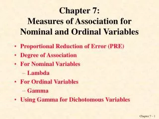
Chapter 7: Measures of Association for Nominal and Ordinal Variables. Proportional Reduction of Error (PRE) Degree of Association For Nominal Variables Lambda For Ordinal Variables Gamma Using Gamma for Dichotomous Variables. Measures of Association.

E N D
Chapter 7:Measures of Association for Nominal and Ordinal Variables • Proportional Reduction of Error (PRE) • Degree of Association • For Nominal Variables • Lambda • For Ordinal Variables • Gamma • Using Gamma for Dichotomous Variables
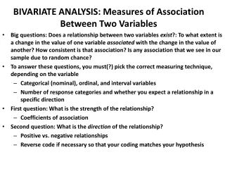
Measures of Association • Measure of association—a single summarizing number that reflects the strength of a relationship, indicates the usefulness of predicting the dependent variable from the independent variable, and often shows the direction of the relationship.
Take your best guess? If you know nothing else about a person except that he or she lives in United States and I asked you to guess his or her race/ethnicity, what would you guess? The most common race/ethnicity for U.S. residents (e.g., themode)! Now, if we know that this person lives in San Diego, California, would you change your guess? With quantitative analyses we are generally trying to predict or take our best guess at value of the dependent variable. One way to assess the relationship between two variables is to consider the degree to which the extra information of theindependent variable makes your guess better.
Proportional Reduction of Error (PRE) • PRE—the concept that underlies the definition and interpretation of several measures of association. PRE measures are derived by comparing the errors made in predicting the dependent variable while ignoring the independent variable with errors made when making predictions that use information about the independent variable.
Proportional Reduction of Error (PRE) where: E1 = errors of prediction made when the independent variable is ignored E2 = errors of prediction made when the prediction is based on the independent variable
Two PRE Measures: Lambda & Gamma • Appropriate for… • Lambda NOMINAL variables • GammaORDINAL & DICHOTOMOUS NOMINAL variables
Lambda • Lambda—An asymmetrical measure of association suitable for use with nominal variables and may range from 0.0 (meaning the extra information provided by the independent variable does not help prediction) to 1.0 (meaning use of independent variable results in no prediction errors). It provides us with an indication of the strength of an association between the independent and dependent variables. • A lower value represents a weaker association, while a higher value is indicative of a stronger association
Lambda where: E1= Ntotal - Nmode of dependent variable
Example 1: 2000 Vote By Abortion Attitudes Table 7.2 2000 Presidential Vote by Abortion Attitudes Abortion Attitudes (for any reason) Vote Yes No Row Total Gore 46 39 85 Bush 41 73 114 Total 87 112 199 Source: General Social Survey, 2002 Step One—Add percentages to the table to get the data in a format that allows you to clearly assess the nature of the relationship.
Example 1: 2000 Vote By Abortion Attitudes Table 7.2 2000 Presidential Vote by Abortion Attitudes Abortion Attitudes (for any reason) Vote Yes No Row Total Gore 52.9% 34.8% 42.7% 46 39 85 Bush 47.1% 65.2% 57.3% 41 73 114 Total 100% 100% 100% 87 112 199 Source: General Social Survey, 2002 Now calculate E1 E1 = Ntotal –Nmode= 199 – 114 = 85
Example 1: 2000 Vote By Abortion Attitudes Table 7.2 2000 Presidential Vote by Abortion Attitudes Abortion Attitudes (for any reason) Vote Yes No Row Total Gore 52.9% 34.8% 42.7% 46 39 85 Bush 47.1% 65.2% 57.3% 41 73 114 Total 100% 100% 100% 87 112 199 Source: General Social Survey, 2002 Now calculate E2 E2 = [N(Yes column total) – N(Yes column mode)] + [N(No column total) –N(No column mode)] = [87 – 46] + …
Example 1: 2000 Vote By Abortion Attitudes Table 7.2 2000 Presidential Vote by Abortion Attitudes Abortion Attitudes (for any reason) Vote Yes No Row Total Gore 52.9% 34.8% 42.7% 46 39 85 Bush 47.1% 65.2% 57.3% 41 73 114 Total 100% 100% 100% 87 112 199 Source: General Social Survey, 2002 Now calculate E2 E2 = [N(Yes column total) – N(Yes column mode)] + [N(No column total) –N(No column mode)] = [87 – 46] + [112 – 73]
Example 1: 2000 Vote By Abortion Attitudes Table 7.2 2000 Presidential Vote by Abortion Attitudes Abortion Attitudes (for any reason) Vote Yes No Row Total Gore 52.9% 34.8% 42.7% 46 39 85 Bush 47.1% 65.2% 57.3% 41 73 114 Total 100% 100% 100% 87 112 199 Source: General Social Survey, 2002 Now calculate E2 E2 = [N(Yes column total) – N(Yes column mode)] + [N(No column total) –N(No column mode)] = [87 – 46] + [112 – 73] = 80
Example 1: 2000 Vote By Abortion Attitudes Table 7.2 2000 Presidential Vote by Abortion Attitudes Abortion Attitudes (for any reason) Vote Yes No Row Total Gore 52.9% 34.8% 42.7% 46 39 85 Bush 47.1% 65.2% 57.3% 41 73 114 Total 100% 100% 100% 87 112 199 Source: General Social Survey, 2002 Lambda = [E1– E2] / E1 = [85 – 80] / 85 = .06
Example 1: 2000 Vote By Abortion Attitudes Table 7.2 2000 Presidential Vote by Abortion Attitudes Abortion Attitudes (for any reason) Vote Yes No Row Total Gore 52.9% 34.8% 42.7% 46 39 85 Bush 47.1% 65.2% 57.3% 41 73 114 Total 100% 100% 100% 87 112 199 Source: General Social Survey, 2002 Lambda = .06 So, we know that six percent of the errors in predicting the relationship between vote and abortion attitudes can be reduced by taking into account the voter’s attitude towards abortion.
EXAMPLE 2: Victim-Offender Relationship and Type of Crime: 1993 Step One—Add percentages to the table to get the data in a format that allows you to clearly assess the nature of the relationship. *Source: Kathleen Maguire and Ann L. Pastore, eds., Sourcebook of Criminal Justice Statistics 1994., U.S. Department of Justice, Bureau of Justice Statistics, Washington, D.C.: USGPO, 1995, p. 343.
Victim-Offender Relationship & Type of Crime: 1993 Now calculate E1 E1 = Ntotal –Nmode = 9,898,980 – 5,045,040 = 4,835,940
Victim-Offender Relationship & Type of Crime: 1993 Now calculate E2 E2 = [N(rape/sexual assault column total) – N(rape/sexual assault column mode)] + [N(robbery column total) –N(robbery column mode)] + [N(assault column total) –N(assault column mode)] = [472,760 – 350,670] + …
Victim-Offender Relationship and Type of Crime: 1993 Now calculate E2 E2 = [N(rape/sexual assault column total) – N(rape/sexual assault column mode)] + [N(robbery column total) –N(robbery column mode)] + [N(assault column total) –N(assault column mode)] = [472,760 – 350,670] + [1,161,900 – 930,860] + …
Victim-Offender Relationship and Type of Crime: 1993 Now calculate E2 E2 = [N(rape/sexual assault column total) – N(rape/sexual assault column mode)] + [N(robbery column total) –N(robbery column mode)] + [N(assault column total) –N(assault column mode)] = [472,760 – 350,670] + [1,161,900 – 930,860] + [8,264,320 – 4,272,230] = 4,345,220
Victim-Offender Relationship and Type of Crime: 1993 Lambda = [E1– E2] / E1 = [4,835,940 – 4,345,220] / 4,835,940 = .10 So, we know that ten percent of the errors in predicting the relationship between victim and offender (stranger vs. non-stranger;) can be reduced by taking into account the type of crime that was committed.
Asymmetrical Measure of Association • A measure whose value may vary depending on which variable is considered the independent variable and which the dependent variable. • Lambda is an asymmetrical measure of association.
Symmetrical Measure of Association • A measure whose value will be the same when either variable is considered the independent variable or the dependent variable. • Gammais a symmetrical measure of association…
Before Computing GAMMA: • It is necessary to introduce the concept of paired observations. • Paired observations – Observations compared in terms of their relative rankingson the independent and dependent variables.
Tied Pairs • Same order pair (Ns) – Paired observations that show a positive association; the member of the pair ranked higher on the independent variable is also ranked higher on the dependent variable.
Tied Pairs • Inverse order pair (Nd) – Paired observations that show a negative association; the member of the pair ranked higher on the independent variable is ranked lower on the dependent variable.
Gamma Gamma—a symmetrical measure of association suitable for use with ordinal variables or with dichotomousnominal variables. It can vary from 0.0 (meaning the extra information provided by the independent variable does not help prediction) to 1.0 (meaning use of independent variable results in no prediction errors) and provides us with an indication of the strength and direction of the association between the variables. When there are more Ns pairs, gamma will be positive; when there are more Nd pairs, gamma will be negative.
Interpreting Gamma The sign depends on the way the variables are coded: + the two “high” values are associated, as are the two “lows” – the “highs” are associated with the “lows” .00 to .24 “no relationship” .25 to .49 “weak relationship” .50 to .74 “moderate relationship” .75 to 1.00 “strong relationship”
Measures of Association • Measures of association—a single summarizing number that reflects the strength of the relationship. This statistic shows the magnitude and/or direction of a relationship between variables. • Magnitude—the closer to the absolute value of 1, the stronger the association. If the measure equals 0, there is no relationship between the two variables. • Direction—the sign on the measure indicates if the relationship is positive or negative. In a positive relationship, when one variable is high, so is the other. In a negative relationship, when one variable is high, the other is low.