Download

1 / 32
330 likes | 354 Vues
This chapter delves into analyzing the relationships between variables at the nominal and ordinal levels using contingency table analysis. Learn how to set up and interpret contingency tables to understand the connections between different variables. Discover the importance of collapsing percentage distributions for clearer interpretations and effective communication in data analysis.

E N D
Part 5: Analysis of Nominal and Ordinal Data Chapters 15, 16, 17
Introduction • Up until now we have examined the treatment of single variables that can be used to describe and summarize • Three levels of measurement (nominal, ordinal, and interval) • Measures of central tendency • This information provides a useful guide to univariate statistics, it is not away enough • Example: An Avery County, California department has just finished conducting its annual survey of public opinion about the agency. • Some of the initial results show that most of the people interviewed now feel that the agency is doing a “very poor job,” and the median opinion is not very optimistic (a “poor job”), • We would like to know not only the distribution of variable scores, but also the explanation for this distribution. Is there a relationship between: • The county of residence of a citizen involved and attitude toward the agency? • The citizens’ attitudes toward the new director and their attitudes toward the agency? • In other words, do the responses on one variable help explain or account for responses on a second variable?
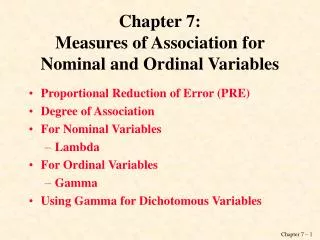
Introduction • Chapter 15 is concerned with relationships between variables measured at the nominaland ordinal levels. • The method that is generally employed to examine these relationships is called contingency table analysis (analysis of cross-tabulations). • Relationships between intervallevel variables are the subject of Regression Analysis (Part VI). • Today we look at how to: • Set up a contingency table; cross-tabulating the responses to a pair of nominal or ordinal variables • Interpret the table or cross-tabulating the responses . • Chapters (16 & 17) will speak more on this topic: • Chapter 16 presents aids to the interpretation of contingency tables • Such as “measures of association” between variables. • Today we will look at the chi-square test of chapter 16. • Chapter 17 discusses a procedure called control table analysis, or statistical controls, • Via this technique the relationships among three or more variables can be examined.
Percentage Distributions • Question: Are there too many federal bureaucrats? • A contingency table is actually a bivariate (two-variable) percentage (or frequency) distribution (Chapter 4). • It tabulates the percentage associated with each data value or group of data values. • Table 15.1 (Response & Frequency) is difficult to interpret. • Table 15.2 & 15.3 facilitates interpretation and comparison.
Collapsing Percentage Distributions • Public Administrators collapse (combine) , a number of original response categories to attain a smaller number of new categories, which are then calculated to yield percentages based on the newly collapsed categories. • Calculating percentage of the newly collapsed categories • Example: Is there are too many federal bureaucrats? “Strongly agree” = 27.0% & “agree”=38.5%; The new collapsed category of “agree” = 65.5% • If a category is not combined with another (non-collapsed) retain the original percentages for those response categories (i.e., Neutral =8.2.)
Collapsing Percentage Distributions • Two primary reasons for presenting the percentage distribution in collapsed form: • It is easier to interpret a distribution based on a few response categories than one based on many. • Defers necessary information to administrators without unnecessary complexity. • Data analyst/manager may not be confident that the distinction between some response categories is very clear or meaningful; • The administrator is more confident that 65.5% of interviewed participants agree with a proposition, more so than exactly 27.0% “strongly agree” and exactly 38.5% “agree.” • Avoids communicating a false sense of precision; contingency tables are based on this format • When you collapse response categories of a variable, the collapsing must not pervert the meaning of the original categories. Response categories can be collapsed only if close in substantive meaning.
Collapsing Percentage Distributions • Major exception to this rule occurs in distributions of nominal variables that have many response categories. • Often only a few of the categories will have a large percentage of cases and most of the other categories will have only trivial numbers. • Here the analyst choose to present: • Each of the categories containing a sizeable percentage • One category labeled “other,” (collapsing all the remaining trivial categories). • Example, the variable is “religion” and the distribution of religion is: • 62% Protestant, 22% Catholic, 13% Jewish, 1% Shinto, 0.5% Buddhist, 0.6% Hedonist, 0.5% Janist, & 0.4% Central Schwenkenfelter • Analyst summarizes this distribution as shown in the adjacent table (15.5);
Collapsing Percentage Distributions • Shawnee Heights Independent Transit Authority has commissioned a poll of 120 persons to determine where Shawnee citizens do most of their shopping. Info is to determine Shawnee Heights future transit routes • The transit planners receive the data shown in the table below (15.6).
Contingency Table Analysis Analysis of contingency tables (cross-tabulations) is the primary method researchers use to examine relationships between ordinal and nominal variables The remainder of the lecture we will cover the construction and interpretation of contingency tables. The methods for percentaging is significant for this type of analysis.
Constructing Contingency Tables • A contingency table or cross-tabulation is a bivariate frequency distribution. • We have dealt with univariate frequency distribution (single-variable). This distribution has a number of cases (or frequency) in which each has a value for a given variable. • A bivariate (two-variable) frequency distribution presents the number of cases that fall into each possible pairing of the values or categories of two variables simultaneously. • Consider the cross-tabulation of the variables “race” (white, nonwhite) and “sex” (male, female) for volunteers to the Klondike Expressionist Art Museum. • There are four possible pairings: white & male, white & female, nonwhite & male, and nonwhite & female volunteers. Pairings across variables are easier to conceptualize if we first consider what the data look like prior to being summarized in a contingency table. • For the Klondike volunteers, gender and race are coded as follows:
Constructing Contingency Tables • The sex and race variables are measured at the nominal level. The raw data for 12 volunteers at the Art Museum is presented in the adjacent table (15.7) • The 1st row of data indicates a score of “1” for both variables (white female). • The 2nd row of data has values of “2” for both variables(nonwhite male). • Interpret the entries for volunteers 3 through 12.
Constructing Contingency Tables • The contingency table displayed below (15.8) is called a cross-tabulation because it crosses (and tabulates) each of the categories of one variable (Sex) with each of the categories of a second variable (Race). • All 451 volunteers at the Art Museum displays the number of cases (volunteers) that fall into each of the race–sex combinations. • The numbers in each cell category simply represent the aggregate results compiled from all 451 rows of data on volunteers, where each row corresponds to a volunteer. • Remember : • That the table may contain large numbers that “look” like interval-level data, but these numbers represent total case counts for nominal- or ordinal-level variables. • The data used to generate Table 15.8 look just like the data for the 12 volunteers displayed in Table 15.7, except that the data for all 451 rows (volunteers) are counted and summarized in Table 15.8. Contingency Table: Race & Sex of Volunteers to Klondike Expressionist Art Museum
Constructing Contingency Tables • Terminology • Cell (Cell frequencies )-The cross-classifications of the two variables—white-male, white-female, nonwhite-male, nonwhite-female. Cell frequencies indicate the number of cases fitting the description specified by the categories of the row and column variables. • Marginals (marginal frequencies) - The total number of respondents who are male or female is presented at the far right of the respective rows. The name is in reference to their position around the perimeter of the table, These totals are calculated by adding the frequencies in the appropriate column or row. • The grand total—the total number of cases represented in the table (N)—is displayed conventionally in the lower right corner of the table. Can be determined by Total of the cell frequencies or the row marginals + column marginals. Contingency Table: Race & Sex of Volunteers to Klondike Expressionist Art Museum
Relationships between Variables • Researchers assemble and examine cross-tabulations because they are interested in the relationship between two ordinal- or nominal-level variables. • A statistical relationship are recognizable pattern of change in one variable as it relates to the change in the other variable. • The type of question that is usually asked is: As one variable increases in value, does the other also increase or does in decrease? • The cell frequencies of a cross-tabulation yield some information about whether changes in one variable are linked statistically with changes in the other variable. • The cross-tabulation presented in the table below (15.10 ), of “education” versus “performance on the civil service examination” exemplify this idea. • Four times as many with high education than low education, but only twice as many of high education got low scores on the civil service exam Relationship b/t Educational Level & Performance on Civil Service Examination
Relationships between Variables • The contingency table analysis process has three major steps that assist with avoiding faulty interpretation. • The problem with the initial interpretation of the contingency table (analysis & understanding) is overlooking the relative number of cases (the marginal totals). This problem can be remedied by percentaging the table appropriately. Steps in the analysis process: • Step 1: Determine which variable is independent and which is dependent. • The independent variable (causal variable) that effects the dependent or response (criterion) variable. • Stated as a hypothesis: The higher the education, the higher the expected score on the civil service examination. Hence, education is the independent variable, and performance on the civil service examination is the dependent variable. • Step 2: Calculate percentages within the categories of the independent variable “education” (independent variable) and the percentages of dependent variable “civil service exam performance (scores). • It’s possible to compare percentages and determine if those with high ed. receive higher scores on the examination than those with low ed. • Allows us to evaluate if the expectation (hypothesis) stated is correct; education leads to improved scores on the civil service examination.
Relationships between Variables • We are interested first in the percentage of people with high school education or less who received high scores on the civil service examination (250). • 150 (60%) received high scores on the test with low education • 100 (40%) of the 250 people with low education received low scores on the test • Moving to those with more than a high school education • 800 (80%) of the 1,000 people with this level of education high scores on the civil service examination. Probability = 0.80 for receiving a high score • 200 (20%) earned low scores. Probability = 0.20 of receiving a low score • Step 3: Compare the percentages calculated within the categories of the independent variable(education) for one of the categories of the dependent variable (performance on the civil service examination).
Relationships between Variables • Our hypothesis is supported by these data: the higher the education, the higher is the score on the civil service examination. • To summarize the relationship between two variables in a cross-tabulation, researchers often calculate a percentage difference across one of the categories of the dependent variable. • In this case, the percentage difference is equal to 80% minus 60%, or 20 percentage points (the percentage of those with high education who earned high scores on the test minus the percentage of those with low education who did so). • Conclusion: Education appears to make a difference of 20 percentage points in performance on the civil service examination. • The percentage difference is a measure of the strength of the relationship between two variables.
Example: Automobile Maintenance in Berrysville • The city council of Berrysville, California, has been under considerable pressure to economize. Last year, the council passed an ordinance authorizing an experimental program for the maintenance of city-owned vehicles. • The bill stipulates that for 1 year out of the city’s 400 automobiles a random sample of: • 150 will receive no preventive maintenance and will simply be driven until they break down. • 250 will receive regularly scheduled preventive maintenance. • The council is interested in whether the expensive program of preventive maintenance actually reduces the number of breakdowns. • After a year under the experimental maintenance program, the city council was presented with the data in table (15.12) on the next slide, which summarizes the number of automobile breakdowns (no maintenance versus preventive maintenance conditions).
Example: Automobile Maintenance in Berrysville • The city council of Berrysville, California, has been under considerable pressure to economize. Last year, the council passed an ordinance authorizing an experimental program for the maintenance of city-owned vehicles. • The bill stipulates that for 1 year out of the city’s 400 automobiles a random sample of: • 150 will receive no preventive maintenance and will simply be driven until they break down. • 250 will receive regularly scheduled preventive maintenance. • The council is interested in whether the expensive program of preventive maintenance actually reduces the number of breakdowns. • After a year under the experimental maintenance program, the city council was presented with the data in table below (15.12), which summarizes the number of automobile breakdowns (no maintenance versus preventive maintenance conditions). Automobile Maintenance Data
Example: Automobile Maintenance in Berrysville • Step to analyze the data for the city council and making a recommendation regarding whether the program should be continued, expanded or terminated. • Step 1: Determine which variable is independent and which is dependent. • “Maintenance” (independent variable), and “breakdowns” (dependent variable). • Stated the hypothesis: The greater the level of maintenance, the less the rate of breakdowns. • Step 2: Calculate percentages within the categories of the independent variable, “automobile maintenance.” The calculations are shown in the table below (15.13). • Step 3: Compare percentages for one of the categories of the dependent variable. • Automobile maintenance appears to make nearly a 30% difference in the rate of breakdowns (difference of 29.6% (52% – 22.4%). • The data show support for the hypothesis: As maintenance increases, the number of breakdowns decreases by almost 30%. From these data, should you recommend to the city council that it continues or terminates the experimental maintenance program? Percentage Distribution for Automobile Maintenance Data
Larger Contingency Tables Relationship between Income and Job Satisfaction • Thus far the contingency tables presented have consisted of “two-by-two” tables (cross-tabulations of independent & dependent variables) • Cross-tabulations can have a greater number of response categories like that found in the adjacent table (15.14) • “How satisfied are you with your job? (Maslow City Post Office employees). • Cross-tabulation of: • Income • Job satisfaction • You would expect income to lead to job satisfaction Table 15.15 presents the cross-tabulation, percentaged
Larger Contingency Tables • The final step in the analysis of contingency tables is to compare percentages for one of the categories of the dependent variable. • The choice of a category in two-by-two tables is not a critical decision, both categories of the dependent variable will yield the same percentage difference • In larger tables, the selection of a category of the dependent variable for purposes of percentage comparison requires more care. • You should not choose an intermediate category, such as “medium” job satisfaction, for this purpose. Choosing either of the endpoint categories—“low” or “high” job satisfaction—will result in clearer understanding and interpretation of the contingency table.
Larger Contingency Tables • Once the (endpoint) category of the dependent variable has been selected, compare the percentages calculated for the endpoint categories of the independent variable. • Avoid intermediate categories of the independent (and dependent) variable for this purpose. • In Table 15.15, this rule suggests that we compare the percentage of those with low income who have high job satisfaction (20%) with the percentage of those with high income who have high job satisfaction (66.7%). • Alternatively, we could compare the percentage of those with low income who express low job satisfaction (50%) with the percentage of those with high income who express low job satisfaction (13.3%).
Larger Contingency Tables • Which percentage comparison(s) should the researcher use to summarize the relationship found in the cross-tabulation? The percentage difference calculation yields different results depending on the endpoint category of the dependent variable chosen. • In the current case, the percentage difference based on high job satisfaction is 66.7% – 20.0% = 46.7%, whereas the percentage difference for low job satisfaction is 50.0% – 13.3% = 36.7%. These percentage differences suggest varying levels of support for the relationship. • Probably the best course of action for the public or nonprofit manager is to consider and report both figures. It shows: • Those with high income have high job satisfaction more often than did those with low income (by 47%) • Those with low income have low job satisfaction more often than did their counterparts with high income (by 37%). • Thus, income appears to make a difference of 37 to 47 percentage points in job satisfaction. • Support the hypothesis: greater the income, greater the job satisfaction.
Displaying Contingency Tables • A set of conventions has been developed for presenting contingency tables. • Contingency tables are rarely presented as bivariate frequency distributions. • You should display the table in percentaged form; the percentages should be calculated and displayed according to the procedures described in the preceding section (do not show the percentage calculations). • The independent variable is placed along the columns of the table, and the dependent variable is positioned down the rows. • Third, the substantive meaning of the categories of the independent variable should show a progression from least to most moving from left to right across the columns, and the categories of the dependent variable should show the same type of progression moving down the rows. • Categories should be listed in the order “low,” “medium,” and “high”; or “disapprove,” “neutral,” and “approve”; or “disagree,” “neutral,” and “agree”, etc.. This facilitates the interpretation of measures of association
Displaying Contingency Tables • A set of conventions has been developed for presenting contingency tables. • The percentages calculated within categories of the independent variable are summed down the column, and the total for each category is placed at the foot of the respective column. • The sum should equal 100%, but because of rounding error, it may vary between 99% and 101%. • Do not add the percentages across the rows of the table; this is a meaningless operation. • The total number of cases within each category of the independent variable is presented at the foot of the respective column. • Usually, these totals are enclosed in parentheses and contain the notation n =_______.
Displaying Contingency Tables • Two problems arise regarding the conventional display of contingency tables. • First, rules are widely accepted—but not always. • In reading and studying contingency tables presented in books, journals, reports, memoranda, magazines, newspapers, etc., don’t assume that the independent variable is always along the columns or that the dependent variable is always down the rows. • Nor can you assume that the categories of the variables are ordered in the table according to the conventions. • Examine the table critically, decide: • Which variable is independent and which is dependent • Whether the percentages have been calculated within the categories of the independent variable, and if the author has compared percentages appropriately. • You should recognize these procedures as the steps specified for analyzing and interpreting cross-tabulations presented in this chapter. Cultivating this habit will not only increase your understanding of contingency table results but also sharpen your analytical skills.
Displaying Contingency Tables • Two problems arise regarding the conventional display of contingency tables. • Second, problem arises as a consequence of computer utilization. • Dealing with contingency tables constructed and percentaged by a computer you may find that computer may be insensible to the distinction between independent and dependent variables, the ordering of response categories of variables • Also computers are usually programmed to print out three different sets of percentages, percentages calculated: • (1) within the categories of the row variable; • (2) within the categories of the column variable • (3) according to the total number of cases represented in the contingency table, sometimes called corner or total percentaging. It is up to you as the data analyst to determine which set of percentages is most meaningful and, if necessary, to reconstruct the contingency table by hand from the computer printout according to the conventional form
Displaying Contingency Tables • This chapter has elaborated a general method for determining whether two variables measured at the nominal or ordinal level are related statistically: contingency table analysis or cross-tabulation. • However, it has not addressed the question of how strongly two variables are related. This question serves as the focus for the next chapter.
Chapter 15 In-Class Problem • 15.1 The Lebanon postmaster suspects that working on ziptronic machines is the cause of high absenteeism. More than 10 absences from work without business-related reasons is considered excessive absenteeism. A check of employee records shows that 26 of the 44 ziptronic operators had 10 or more absences and 35 of 120 nonziptronic workers had 10 or more absences. Construct a contingency table for the postmaster. Does the table support the postmaster’s suspicion that working on ziptronic machines is related to high absenteeism?
Absenteeism Due to Ziptronic • The percentage difference between Ziptronic Workers and Non-Ziptronic Worker that experience 10 or more non-business related absences is 29.9%, in favor of Ziptronic Workers • The percentage difference between Ziptronic Workers and Non-Ziptronic Worker that experience < 10 non-business related absences is 29.9%, in favor of Non-Ziptronic Workers.