Download

1 / 38
400 likes | 626 Vues
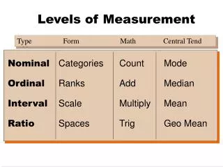
Four levels of measurement. Nominal: the lowest level Ordinal Interval Ratio: the highest level. Ratio. Interval. Ordinal. Nominal. Classic Parametric Setting.

E N D
Four levels of measurement • Nominal: the lowest level • Ordinal • Interval • Ratio: the highest level Ratio Interval Ordinal Nominal
Classic Parametric Setting For the classic ANOVA, we assume we are sampling from normally distributed populations with identical variances. From here we test the hypothesis: H(0):μ1= μ2 = μ3 (All distributions are identical) or μ1- μ overall = 0, μ2 - μ overall = 0, μ3 - μ overall =0
Nonparametric Setting H(0): F0 = F2 = F4 = F6 = F8 (Identical Distributions) or F0 - H = 0, F2 - H = 0, F4 - H = 0, F6 - H = 0, F8 - H = 0 where H is the overall average distribution.
Settings for Nonparametric Tests • When data are very non-normal (e.g. very skewed, or presence of outliers) • If you suspect the variable is not normally distributed in the population • When you have ordinal data and are interested in comparing distributions and their relationships. • If other assumptions of parametric tests are violated (e.g. homogeneity of variance, ordinal • data)
Nonparametric Methods • Can provide invariant results when strictly monotone transformations of the data are used.
Gamma GT Study Note Non Constant Variance, Outliers, and Heavily Skewed Distributions
Gamma GT Means Original data means, means of ln(x), and means of ln(ln(x)). Note reversal of treatment means. Nonparametric gives same result for all 3 ‘versions’ of the data
Nonparametric Methods • Absence of variability in treatment groups is admitted
Panic 2 Study. Note skewed distributions, outliers, and zero variance at Week 10.
Nonparametric Methods • Can provide approximations for small sample sizes
Nonparametric Methods • Can be performed using SAS macros • “Proc Mixed”
Disadvantages - Advantages • Lesser power relative to corresponding parametric test (when assumptions of the parametric test are met) • When assumptions of parametric tests are not met nonparametric methods can be more powerful
Definition of Probability ‘Distributions’ Probability Distribution Function (f): A function that assigns a probability to each possible outcome. P(X = Some particular set of values of x) for all possible x Cumulative Probability Distribution Function (F): A function that assigns a probability to a value less than or equal to each possible outcome. P(X some particular value of x) for all possible x
Empirical Distribution Function F If we have a sample from a ‘Parent Distribution’ F, our estimate of F from the sample is the Empirical Distribution Function, denoted F hat.
Relative Effects P(i) The empirical distribution functions F(i), do provide information to detect differences among the different group distributions. But there exists a summary measure that describes the likelihood that values from one distribution tend to be greater or lesser than the overall mean distribution H. This measure is called: the ‘Relative Effect’ for group i.
Interpretation of Relative Effects p(i) The relative effect p(i) quantifies the tendency of the marginal distribution F(i) with respect to the overall average distribution H. If F(i) tends to lie in the region to the left of H then p(i) < 0.5. If F(i) tends to lie in the region to the right of H then p(i) > 0.5.
Calculation of Estimated Relative Effects: A function of the ranks
The Relationship of the Distribution function F(i), p(i), and μ (i)
Covariance Matrix Notes: 1. A covariance matrix must have an inverse in order to calculate many multivariate stats (Wald, Hotelling). 2. A covariance matrix of a set of variables in which one variable has ZERO variance will not have an inverse. 3. Both of the above types of covariance matrices have a TRACE, the sum of the diagonal elements.
Relative Effects P(i) The empirical distribution functions F(i), do provide information to detect differences among the different group distributions. But there exists a summary measure that describes the likelihood that values from one distribution tend to be greater or lesser than the overall mean distribution H. This measure is called: the ‘Relative Effect’ for group i.
Interpretation of Relative Effects p(i) The relative effect p(i) quantifies the tendency of the marginal distribution F(i) with respect to the overall average distribution H. If F(i) tends to lie in the region to the left of H then p(i) < 0.5. If F(i) tends to lie in the region to the right of H then p(i) > 0.5.
Calculation of Estimated Relative Effects: A function of the ranks
The Relationship of the Distribution function F(i), p(i), and μ (i)
data panic1; input patient t1-t5; array t{5} t1-t5; do i=1 to 5; week=(i-1)*2; score=t{i};output; end; drop i t1-t5; datalines; 1 8 6 5 5 4 2 8 6 5 4 2 3 6 5 5 4 2 4 6 6 6 5 5 5 7 6 6 6 6 6 8 7 3 2 2 7 7 6 7 3 3 8 6 4 5 3 3 9 5 4 3 3 2 10 8 6 5 5 4 11 7 6 5 4 2 12 6 5 5 4 2 13 6 6 6 5 5 14 8 6 6 6 6 15 8 7 4 2 2 16 7 6 7 3 3 ; run;
Obs patient week score 1 1 0 8 2 1 2 6 3 1 4 5 4 1 6 5 5 1 8 4 6 2 0 8 7 2 2 6 8 2 4 5 9 2 6 4 10 2 8 2 . . . . . . . . . . . . 71 15 0 8 72 15 2 7 73 15 4 4 74 15 6 2 75 15 8 2 76 16 0 7 77 16 2 6 78 16 4 7 79 16 6 3 80 16 8 3
%include'E:\nonparametric\SAS Macros\ld_f1.sas'; %ld_f1(data=panic1, var=score, time=week, subject=patient, var_pt=_no_, time_pt=_no_); run; %include'E:\nonparametric\SAS Macros\ld_ci.sas'; %ld_ci(data=panic1, var=score, time=week, subject=patient, alpha=0.05); run;
LD_1F --- subjects x T T: fixed, subjects: random SAS-data-filename: panic1 response-variable: score Class Level Information CLASS LEVELS T WEEK 5 Total number of observations 80 Total number of subjects 16 Number of missing values 0 RTE = relative treatment Effects Nobs = Number of observations (do not count the repeated measurements within the cells)
Source Time Rank means Nobs RTE week 0 66.094 16 .81992 week 2 50.500 16 .62500 week 4 41.281 16 .50977 week 6 25.625 16 .31406 week 8 19.000 16 .23125 The SAS System 10 17:29 Friday, October 3, 2003 ---------------------------------------------------------- Statistics df1 df2 p-value Wald Chi^2(df1) 126.69 4.0000 . .00000 Hotelling F(df1,df2) 25.339 4.0000 12.000 .00001 Anova Chi^2(df1)/df1 36.937 2.2341 . .00000
The SAS System 11 17:29 Friday, October 3, 2003 LD_CI Bias-Estimation and Confidence-Intervals for Relative Effects SAS-Data-Filename: panic1 Response-Variable: score Observations: 80 Group-Variable: _none_ Groups: 1 Time-Variable: week Timepoints: 5 Subject-Variable patient Subjects: 16 Relative Effects, Biases, Variances and Confidence-Limits (alpha=0.05) Time RE Bias Variance lower upper 0 .81992 .00284 .00768 .76566 .85379 2 .62500 -.0008 .01571 .56079 .68278 4 .50977 .00310 .02512 .43271 .58610 6 .31406 -.0018 .00800 .27316 .36061 8 .23125 -.0033 .01597 .18033 .30524