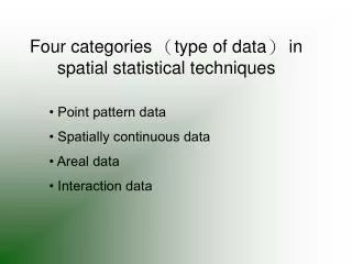
Four categories ( type of data ) in spatial statistical techniques
400 likes | 595 Vues
Four categories ( type of data ) in spatial statistical techniques. • Point pattern data • Spatially continuous data • Areal data • Interaction data. Three measurement scales. Nominal Simply identify different categories ( e.g. 1=females, 2=males ). Ordinal

Four categories ( type of data ) in spatial statistical techniques
E N D
Presentation Transcript
Four categories (type of data) in spatial statistical techniques • Point pattern data • Spatially continuous data • Areal data • Interaction data
Three measurement scales • Nominal • Simply identify different categories (e.g. 1=females, 2=males). • Ordinal • The numbers imply an ordering in the categories (e.g. 1=very good, 2=quite good, 3=medium, 4=poor). However, the numbers cannot be added, subtracted, multiplied or divided in any meaningful way. • Interval • interval scale measure quantity (e.g. temperatures in degrees Centigrade). This means that the difference (i.e.interval) between two values is a measure of quantity.
Classification of statistical techniques (depending upon the purpose ) • Visualization:This simply refers to plots, graphs, maps and various other ways of graphical depicting the data. • Exploration: The objective here is to describe the data. This may involve the calculation of descriptive statistics (e.g. mean, standard deviation) or it may involve a form of visualization after further processing of the data. • Modeling:The objective here is to examine relationships or quantify descriptive parameters in a more formal manner. Modeling is involved in all forms of statistical inference or hypothesis testing, although this fact may be disguised in the simpler ‘cookbook’ statistics texts. • Statistical modeling visualization explored in more detail in the following Modeling
MODELLING SPATIAL DATA(Basic Concepts) • Since statistical models are concerned with phenomena which are stochastic, that is to say phenomena which are subject to uncertainty, or governed by the laws of probability, we need a 'language' which allows us to represent such uncertainty mathematically. This is provided by the concept of a random variable and its associated probability distribution.
函數表示法 The relative chance of a random variable taking different possible values is characterized by its associated probability distribution, so that we might refer to the random variable Y as having a probability distribution fY(y). fY(y) is a mathematical function which specifies the probability that Y has the specific value (or ranges of values) y. The random variables are represented by upper case letters, and specific values of a random variable by lower case letters. For example, Y may be a random variable that conceptually represents the result of throwing a die, but when it is actually thrown we get a particular observed value y of this random variable.
分立與連續變項之機率分布 • random variables may be discrete, that is, only able to take a finite number of values; in this case fY(y) is the probability that Y takes the specific value y. • They may also be continuous, able to take any value within a continuous range, in which case fY(y) is the probability density at the value y.
機率公式 • The probability that a random variable Y takes values in some range (a, b) is therefore:
累積機率分布 We may also occasionally be interested in the cumulative probabilitydistribution FY(y) of a random variable Y, sometimes referred to as its distribution function. This is simply a mathematical function which specifies the probability that Y takes any value less than or equal to the specific value y. Thus:
期望值(平均值) • Expected value or mean, of a random variable Y, or perhaps some function, g(Y), of that random variable. As its name suggests, this is simply the 'average' value that we would expect Y or g(Y) to take. It is therefore a weighted sum of the possible values, where the weights used for each value are the probability associated with that value. Therefore: or
變異數 • The expected value of one particular function of a random variable is often of particular interest, namely the expected squared deviation of the random variable from its mean. This is the variance of the random variable and it is a broad measure of how much its values tend to vary around their 'average'. Formally, VAR(Y) = ([Y - E(Y)]2).
標準差 • The positive square root of this quantity is referred to as the standard deviation of the random variable.
共變數 • All of these ideas generalize to the case where we are interested not just in one random variable but in more than one. If we have two random variables (X, Y), then we can speak of their joint probability distribution, fXY(x,y), which specifies the probability, or probability density, associated with X taking the specific value x, at the same time that Y takes the specific value y. As well as the mean and variance of Y or X, we may then also be interested in the expected tendency for values of X to be 'similar' to values of Y. A broad measure of this is the covariance of the two random values, defined as COV(X,Y) = (((X - E(X)).(Y - E(Y))). The covariance of two random variables divided by the product of their standard deviations is referred to as the correlation between them.
獨立性 • Two random variables are said to be independent if the probabilistic behavior of either one remains the same, no matter what values the other might take. In that case their joint probability distribution is simply the product of their individual probability distributions, so that fXY(x,y)=fX(x)fY(y). If this is so then it follows that their covariance and correlation will be zero.
Statistical Models –以擲骰子、ozone為例 • Simple, like throwing a die, which involves a single random variable, say Y, this means specifying a corresponding probability distribution, fY(y). • More complex phenomena, for example modeling levels of a photochemical oxidant such as ozone in a large rural region. The ozone level at each location, s, in the region R, will vary during the course of a day and from day to day according to some probability distribution.
Note that s is a (2 x 1) vector = (s1,s2)T which refers to a point location, where T indicates the matrix should be transposed – i.e. it is a column vector. This is simply a shorthand way of referring to the x-coordinate s1 and the y-coordinate s2 of a point. The bold typeface indicates a vector. If we have two point locations we can refer to them by the two vectors s1 and s2 where s1=(s11,s12)T and s2=(s21,s22)T.
空間隨機分布 • The particular form of the ozone level probability distribution may well differ from location to location in R. Furthermore the ozone levels at neighboring locations may well be related in some way. For example, ozone levels at sites separated by 5 kilometers are probably quite similar, while those separated by 50 kilometers may be very different. Thus, to represent ozone levels in R we require a set of possibly non-independent random variables, {Y(s),s R}. Such a set is often referred to as a spatial stochastic process. • A complete statistical model for the ozone level in region R involves specifying the joint probability distribution of every possible subset of these random variables. Without simplifying assumptions, this would be a formidable task.
例子一、擲骰子 • For example, an obvious model for a fair die is: fY(y)=1/6, y=l...6.
例子二、ozone • A typical data set in the ozone level example would consist of a set of observations (y1,y2, …), each at specific sites, (s1,s2, …)in R. This data set, (y1, y2, …), is often referred to as a realizationof the spatial process. It is just one observation from the joint probability distribution of the random variables{Y(s1), Y(s2), …}- or in simpler notation {Y1,Y2, …}. Unfortunately, one observation does not give much information about a joint probability distribution, even if we were prepared to accept that this particular set of sites was 'typical' (i.e. an unbiased sample) of sites in general in R, which may itself be open to question.
資料與假設 -probability distribution,parameters and fitted • The specification of a model generally involves using a combination of both data and 'reasonable' assumptions about the nature of phenomena. Such assumptionsmay arise, for example, from background theoretical knowledge about how one expects a phenomenon to behave, the results of previous analyses on the same, or a similar, phenomenon, or alternatively, from the judgment and intuition of the modeler. How ‘reasonable' these assumptions are, in certain cases, can be assessed by exploratory analyses of aspects of the observed data appropriate to those particular assumptions. Once specified, they provide a basic 'framework' for a model. Usually this framework will amount to the specification of a general mathematical form for the probability distribution appropriate to the phenomenon, but one which involves certainparameters whose values are left unspecified. This general form is then further refined, or fitted (i.e. the values of the unknown parameters are estimated), by reference back to the observed data. The fitted model can then be evaluated, which may lead to modified assumptions and a different model being fitted, and so on.
Standard linear regression model-ozone level example • Widely used in non-spatial analysis • to our ozone level example. A model of this type would involve: • The assumption that the random variables {Y(s), s R} are independent • Probability distributions only differ in their mean value, all other aspects being the same • Mean value is a simple linear function of location, say E(Y(s)) =β0 +β1s1 +β 2s2 where (s1,s2) are the spatial coordinates of the locations; and • Each Y(s) has a normal distribution about this mean with the same constant variance • In short, our model says that Y(s) are independent and the probability distribution of each is N(β0 +β1s1 +β 2s2, σ2) – i.e. normal with mean β0 +β1s1 +β 2s2 and variance σ2.
Parameter Estimation • Maximum likelihood : The idea of maximum likelihood is really quite simple. Our exploratory analyses, background knowledge, intuition and judgment have led us to a model framework, which, as discussed previously, will usually amount to the specification of a general mathematical form for the probability distribution appropriate to the phenomenon under study, but one which involves certain parameters whose values are left unspecified. In general let us denote these unknown parameters by the vector θ. In the above example of the linear regression model, θ would have four elements (β 0, β1, β2 and σ2), but in general it might have any number of elements. Now, if the model framework provides a general mathematical form for the probability distribution appropriate to the phenomenon under study, then from this we must be able to write down a general mathematical form for the joint probability distribution of the set of random variables{Y1, Y2, … Yn} for which our data (y1, y2, … yn) constitute a set of observed values. Suppose that this joint probability distribution is f(y1, y2, … yn; θ). Here we have explicitly indicated that as well as being a function of the observed values (y1, y2, … yn), this will also in general depend on the values of the unknown parameters θ.
θ • How is f(y1, y2, … yn; θ ) to be interpreted? It is a joint probabilitydistribution so, givenparticular values forθ, it specifies the probability, or probability density, associated with Y1 taking the specific value yl at the same time that Y2 takes the specific value y2 and so on. Hence, if (y1, y2, … yn) are our actual data observations, f(y1, y2, … yn; θ)is effectively the probability or probability density associated with them occurring, given the general model framework proposed. We refer to this as the likelihoodfor the data, and we would normally denote it as L(y1, y2, … yn; θ). Notice that given a known set of observed data (y1, y2, … yn), the likelihood depends only on the unknown parameter values θ. Recall that our objective is to estimate values forθand an obvious way of doing this is now apparent. We should choose values for θ that maximize the likelihood for the observed data. Often, because it is easier and equivalent, we maximize the logarithm of the likelihood or the log likelihood, which we denote log(y1, y2, … yn; θ). Under the maximization of either function, we are effectively 'tuning' our proposed model framework by choosing parameter values which give the greatest possible likelihood of observing the data that we actually observed. This would seem a sensible way to proceed.
Ordinary and Generalized Least Squares • This, then, is the general approach to parameter estimation or model fitting, known as maximum likelihood. Of course, in any specific case the maximization of L(y1, y2, … yn; θ) or its logarithm, with respect toθ, may not be particularly easy and may involve intensive computation and the development of algorithms to numerically approximate the solution. However, for some 'standard' and commonly used model frameworks it turns out to be relatively straightforward and mathematically equivalent to ways of fitting models with which you may be more familiar. For example, for the multiple linear regression model discussed earlier, where the model framework involves the assumption of independently distributed random variables, having normal distributions with the same variance, maximum likelihood parameterestimation reduces to using the method of ordinary least squares. That is, parameters are estimated by minimizing the sum of squared 'residuals' or differences between the data values and those predicted under the model. If we relax the assumption of independence and equal variance, but maintain the other aspects of the model, then maximum likelihood leads to parameter estimation by generalized least squares, which is the minimization of a weighted sum of squared 'residuals'.
Parameter Estimate and Model Fit • Maximum likelihoodnot only provides parameter estimates, but alsogeneral measures of how reliable these estimates are (i.e. their standard errors) and of how well alternative models fit a particular set of data. • Standard errors are, in essence, derived by consideration of how 'peaked' the likelihood function is at its maximum. • Informally, the idea is again simple. If the likelihood is highly 'peaked' at its maximum and falls sharply in value as you move away from this, then you can be pretty sure that the estimated parameter values are reasonably reliable (small standard errors). • If, alternatively, the maximum occurs at some point on a slowly changing 'plateau', then the value of the likelihood is similar all over this 'plateau' and therefore for several different sets of parameter values; hence you should be less confident in the estimates derived (large standard errors). • When it comes to comparing the overall fit of two different models we can consider the ratio of the likelihoods associated with each (duly maximized for the parameters involved). Informally, we ask whether one value is significantly better than the other.
Hypothesis Testing • Testing a hypothesis is a question of comparing the fit to the data of two models • one of which incorporates assumptions which reflect the hypothesis • the other incorporating a less specific set of assumptions • Usually a hypothesis will amount to the specification of values for certain of the parameters involved in the model. Testing hypotheses is therefore one facet of statistical modeling • No new theory is really involved, although of course we can wrap all this up in the language of 'p-values' and so on, if we so wish. • Notice, however, that all modelinginevitably involves some assumptions about the phenomenon under study; hence hypothesis testing will always involve comparison of the fit of a hypothesized model with that of an alternative which also incorporates assumptions, albeit of a more general nature. • The validity of a particular form of hypothesis test often relies critically on these alternative assumptions being, in turn, valid for the phenomenon in question. • For example, in the ozone model discussed above, the standard multiple regression test of whether the parameters β1 and β2 are significantly different from zerodepends on both the assumption of the independence of Y(s) and of a normal distribution for these random variables.
Spatial Data Modeling(spatial phenomena) • Spatial phenomena often exhibit a degree of spatial correlation. Spatial analysts need to incorporate the possibility of such spatial dependence into their models if the models are to provide realistic representations of such phenomena. • For example, the independence assumption of the standard multiple regression model would be unlikely to be realistic in relation to our ozone level example. • In addition to the mean value of the ozone level varying in R, • the distribution of values about this mean at any site is likely to be related to that in neighboring sites. • In general the behavior of spatial phenomena is often the result of a mixture of both first order and second order effects. • First order effects relate to variation in the mean value of the process in space – a global or large scale trend. • Second order effects result from the spatial correlation structure, or the spatial dependence in the process; in other words, the tendency for deviations in values of the process from its mean to 'follow' each other in neighboring sites - local or small scale effects.
例子(Random) • Suppose we imagine scattering, entirely at random, iron filings on to a sheet of paper marked with a fine regular grid. • The numbers of iron filings landing in different grid squares can be thought of as the realization of a spatial stochastic process. • As long as the mechanism by which we scatter the filings is purely random, there should be an absence of both first and second order effects in the process • Different numbers of filings will occur in each square, but these differences arise purely by chance.
First and Second Order Effects • Now suppose that a small number of weak magnets are placed under the paper at different points and we scatter the filings again. The result will be a process with spatial pattern arising from a first order effect - clustering in the numbers in grid squares will occur globally at and around the sites of the magnets. • Now removethe magnets, weakly magnetize the iron filings instead, and scatter them again. The result is a process with a spatial pattern arising from a second order effect - some degree of local clustering will occur because of the tendency for filings to attract each other. • If the magnets are now replaced under the paper and the magnetized filings scattered again, we end up with a spatial pattern arising from both first and second order effects.
Because 'real life' spatial patterns frequently arise from this sort of mixture of both first and second order effects, independence in the random variables representing a spatial stochastic process is often too strong an assumption for the spatial modeler. • By definition, such an assumption rules out second order effects and therefore needs to be replaced by some weaker alternative which allows for the possibility of a covariance structure. • A common approach is to think of the variable of interest (such as the ozone level at a location) as comprising two components. • The first order component represents large scale spatial variation in mean value. • This is similar to the dependence proposed in the simple regression model used earlier, although the relationship between the mean and location need not be linear, whilst 'covariates' might be included in the relationship, instead of, or together with, location. • The second order component is concerned with the behavior of stochastic deviations from this mean. • Instead of assuming these to be spatially independent, they are allowed to have a covariance structure which may give rise to local effects.
Covariance • A common approach is to think of the variable of interest (such as the ozone level at a location) as comprising two components. • The first order component represents large scale spatial variation in mean value. • This is similar to the dependence proposed in the simple regression model used earlier, although the relationship between the mean and location need not be linear, whilst 'covariates' might be included in the relationship, instead of, or together with, location. • The second order component is concerned with the behavior of stochastic deviations from this mean. • Instead of assuming these to be spatially independent, they are allowed to have a covariance structure which may give rise to local effects.
The second order component is often modeled as a stationary spatial process. Informally, a spatial process {Y(s),s R} is stationary or homogeneous if its statistical properties are independent of absolute location in R. • In particular, this would imply that the mean, E(Y(s)), and variance, VAR(Y(s)), are constant in R and therefore do not depend upon locations. • Stationarity also implies that the covariance, COV(Y(si),Y(sj)), between values at any two sites, si and sj, depends only on the relative locations of these sites, the distance and direction between them, and not on their absolute location in R. • Further, the spatial process is isotropic if, in addition to stationarity, the covariance depends only on the distance between s1 and s2 and not on the direction in which they are separated.
Nonstationarity( heterogeneity ) • If the mean, or variance, or the covariance structure 'drifts' over R.
鐵砂與磁鐵 • In terms of our earlier example, the case where weakly magnetized iron filings are scattered onto paper with no magnets underneath would roughly equate to an isotropic process. • The case with unmagnified filings and magnets underneath the paper, approximates a process with heterogeneity in the mean value and independence in deviations from mean value - a simple form of non-stationary model, similar in spirit to our simple regression model, although obviously not in respect of the relationship between mean and location, which would be non-linear in this case. • The experiment with both magnetized filings and magnets under the paper is a more complex non-stationary process that mixes the previous two cases and might be considered akin→ a 'two component' model often useful in practice for spatial processes. It involves first order variation or heterogeneity in mean value, combined with a stationary second order effect.
合理簡化 • Heterogeneity in the mean, combined with stationarity in second order effects, is a useful spatial modeling assumption, where it may be regarded as 'reasonable' and acceptable, since it implies that the covariance of the process has the same structure from area to area within the region studied. • If all locations in space have potentially different covariancestructures as well as means, and, as is usual, we have only a set of single observations at a particular subset of locations, then we stand little chance of estimating all parameters involved in the model. • The modeling of a spatial process often tends to proceed by first identifying any heterogeneous 'trend' in mean value and then modeling the 'residuals', or deviations from this 'trend', as a stationary process.
問題 • If high values of a process are found in one region and low values among a set of adjacent sites in another region, then how do we know whether the underlying process is non-stationary (i.e. heterogeneous) or if these are local effects resulting from a homogeneous spatial dependence in the data? • In other words, how can we distinguish spatial dependence in a homogeneous environment from spatial independence in what is a heterogeneous environment? ※ No definitive answers. (Analytical methods can help to identify appropriate models and distinguish in some cases between effects that must clearly be global first order trends and those that are more likely to be the result of a second order covariance structure.)
Ultimately, models are mathematical abstractions of reality and notreality itself. • the specification of a model will always involve using a combination of both data and assumptions about the nature of phenomena being modeled. Ultimately, judgment and intuition on the part of the analyst are always involved in statistical modeling. • Statistical models are always at best 'not wrong', rather than 'right'.
GEOGRAPHICALLY WEIGHTED REGRESSION • The ozone model discussed above models the relationship between ozone levels and location in space - i.e. it does not consider covariates (i.e. other ‘predictor’ variables which might impact upon ozone levels, e.g. traffic levels). Covariates are often incorporate in a multiple regression model taking the general form: Where there are k predictors, xik is the value of variable k at location i, and βk is a parameter indicating the relationship between the dependent variable Y and variable Xk. • This model presupposes that the regression coefficients are homogeneous or stationary - i.e. that the relationship between the dependent variable and each independent (or predictor) variable is the same everywhere. However, this assumption may not be realistic.
GEOGRAPHICALLY WEIGHTED REGRESSION • To accommodate these situations, Fotheringham et al. have proposed a non-stationary model: • the values of the regression coefficients β are a function of location (where ui and vi represent the x and y co-ordinates). • One problem with this model is that there are too many unknown parameters, so it is necessary to introduce simplifying assumptions in order to calibrate the model (i.e. estimate the parameters). Geographically weighted regression (GWR) assumes that the parameters are functions of location (i.e. that they are non-stationary). • Each of the regression coefficients estimated by GWR is a function of location.

![Data Modeling [Comparison of data modeling techniques ]](https://cdn0.slideserve.com/205866/data-modeling-comparison-of-data-modeling-techniques-dt.jpg)