Lorenz Lecture
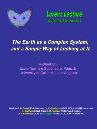
Lorenz Lecture. AGU Fall Mtg., 5 December 2005. The Earth as a Complex System, and a Simple Way of Looking at It. Michael Ghil Ecole Normale Supérieure, Paris, & University of California, Los Angeles. Work with D. Dee (NASA Goddard), V. Keilis-Borok (IGPP, UCLA, & MITP, Moscow),

Lorenz Lecture
E N D
Presentation Transcript
Lorenz Lecture AGU Fall Mtg., 5 December 2005 The Earth as a Complex System, and a Simple Way of Looking at It Michael Ghil Ecole Normale Supérieure, Paris, & University of California, Los Angeles Work with D. Dee (NASA Goddard), V. Keilis-Borok (IGPP, UCLA, & MITP, Moscow), A. Mullhaupt(Wall Street), P. Pestiaux (TotalFina, France), A. Saunders (UCLA), & I. Zaliapin (IGPP, UCLA, & MITP, Moscow).
Edward Norton Lorenz born May 23, 1917 Jule Gregory Charney January 1, 1917 – June 16, 1981
Motivation • Components - solid earth (crust, mantle) - fluid envelopes (atmosphere, ocean, snow & ice) - living beings on and in them (fauna, flora, people) • 2. Complex feedbacks • - positive and negative • - nonlinear - small pushes, big effects? • 3. Approaches • - reductionist • - holistic • 4. What to do? - Let’s see!
F. Bretherton's "horrendogram" of Earth System Science Earth System Science Overview, NASA Advisory Council, 1986
The climate system on long time scales “Ambitious” diagram m T Flow diagram showing feedback loops contained in the dynamical system for ice-mass mand ocean temperature variations T Constants for ODE & PDE models are poorly known. Mechanisms and effective delays are easier to ascertain. B. Saltzman, Climatic system analysis, Adv. Geophys.,25, 1983
Introduction Binary systems Examples: Yes/No, True/False (ancient Greeks) Classical logic(Tertium not datur) Boolean algebra (19th cent.) Propositional calculus (20th cent.) (syllogisms as trivial examples) Genes: on/off Descriptive – Jacob and Monod (1961) Mathematical genetics – L. Glass, S. Kauffman, M. Sugita (1960s) Symbolic dynamicsof differentiable dynamical systems (DDS): S. Smale (1967) Switches: on/off, 1/0 Modern computation (EE & CS) - cellular automata (CAs) J. von Neumann (1940s, 1966), S. Ulam, Conway (the game of life), S. Wolfram (1970s, ‘80s) - spatial increase of complexity – infinite number of channels - conservative logic Fredkin & Toffoli (1982) - kinetic logic: importance of distinct delays to achieve temporal increase in complexity (synchronization, operating systems & parallel computation), R. Thomas (1973, 1979,…)
Introduction (continued) M.G.’s immediate motivation: Climate dynamics – complex interactions (reduce to binary), C. Nicolis (1982) Joint work on developing and applying BDEs to climate dynamics with D. Dee, A. Mullhaupt & P. Pestiaux (1980s) & with A. Saunders (late 1990s) Work of L. Mysak and associates (early 1990s) Recent applications to solid-earth geophysics (earthquake modeling and prediction) with V. Keilis-Borok and I. Zaliapin Recent applications to the biosciences (genetics and micro-arrays) Oktem, Pearson & Egiazarian (2003) Chaos Gagneur & Casari (2005) FEBS Letters
Outline What for BDEs? - life is sometimes too complex for ODEs and PDEs What are BDEs? - formal models of complex feedback webs - classification of major results Applications to climate modeling - paleoclimate – Quaternary glaciations - interdecadal climate variability in the Arctic - ENSO – interannual variability in the Tropics Applications to earthquake modeling - colliding-cascades model of seismic activity - intermediate-term prediction Concluding remarks - bibliography - future work
What are BDEs? Short answer: Maximum simplification of nonlinear dynamics (non-differentiable time-continuous dynamical system) Longer answer: x 1) (simplest EBM: x = T) 0 1 2 3 t x 2) 0 1 2 3 t 3) x1 0 1 1.5 3 4.5 t Eventually periodic with a period = 2(1+q) x2 (simplest OCM: x1=m, x2=T) 0 1 2.5 4 t
q is irrational Increase in complexity! Evolution: biological, cosmogonic, historical But how much? Dee & Ghil, SIAM J. Appl. Math. (1984), 44, 111-126
Aperiodic solutions with increasing complexity Jump Function Time Theorem: Conservative BDEs with irrational delays have aperiodic solutions with apower-law increase in complexity. N.B. Log-periodic behavior!
The geological time scale Ice age begins Earliest life http://www.yorku.ca/esse/veo/earth/image/1-2-2.JPG Density of events
The place of BDEs in dynamical system theory after A. Mullhaupt (1984)
Classification of BDEs Definition: A BDE is conservative if its solutions are immediately periodic, i.e. no transients; otherwise it is dissipative. Remark: Rational vs. irrational delays. Example: 1) Conservative 2) Dissipative Analogy with ODEs Conservative – Hamiltonian Dissipative – limit cycle attractor no transients M. Ghil & A. Mullhaupt, J. Stat. Phys., 41, 125-173, 1985
Examples.Convenient shorthand for scalar 2nd order BDEs 1. Conservative Remarks: i) Conservative linear (mod 2) ii) few conservative connections (~ ODEs) 2. Dissipative Theorem Conservative reversible invertible A. Mullhaupt, Ph.D. Thesis, May 1984, CIMS/NYU M. Ghil & A. Mullhaupt, J. Stat. Phys., 41, 125-173, 1985
Classification of BDEs Structural stability & bifurcations Theorem BDEs with periodic solutions only are structurally stable, and conversely Remark.They are dissipative. Meta-theorems, by example. The asymptotic behavior of is given by Hence, if then solutions are asymptotically periodic; if however then solutions tend asymptotically to 0. Therefore, as q passes through t, one has Hopf bifurcation.
Paleoclimate application: Thermohaline circulation and glaciations Logical variables T - global surface temperature; VN - NH ice volume, VN= V; VS- SH ice volume, VS= 1; C - deep-water circulation index M. Ghil, A. Mullhaupt, & P. Pestiaux, Climate Dyn., 2, 1-10, 1987.
Scalar time series that capture ENSO variability The large-scale Southern Oscillation (SO) pattern associatedwith El Niño (EN), as originally seen in surface pressures Neelin (2006) Climate Modeling and Climate Change, after Berlage (1957) Southern Oscillation: The seesaw of sea-level pressures ps between the two branches of the Walker circulation Southern Oscillation Index (SOI) = normalized difference between ps at Tahiti (T) and ps at Darwin (Da)
Scalar time series that capture ENSO variability Time series of atmospheric pressure and sea surface temperature (SST) indices Data courtesy of NCEP’s Climate Prediction Center Neelin (2006) Climate Modeling and Climate Change
Histogram of size distribution for ENSO events A. Saunders & M. Ghil, Physica D, 160,54–78,2001 (courtesy of Pascal Yiou)
BDE Model for ENSO: Formulation A. Saunders & M. Ghil, Physica D, 160,54–78,2001
Devil's Bleachers in a 1-D ENSO Model F.-F. Jin, J.D. Neelin & M. Ghil, Physica D, 98, 442-465, 1996
Devil's Bleachers in the BDE Model of ENSO A. Saunders & M. Ghil, Physica D, 160,54–78,2001
Colliding-Cascade Model 1. Hierarchical structure 2. Loading by external forces 3. Elements’ ability to fail & heal A. Gabrielov, V. Keilis-Borok, W. Newman, & I. Zaliapin (2000a, b, Phys. Rev. E; Geophys. J. Int.) Interaction among elements
BDE model of colliding cascades: Three seismic regimes I. Zaliapin, V. Keilis-Borok & M. Ghil (2003, J. Stat. Phys.)
BDE model of colliding cascades Regime diagram: Instability near the triple point I. Zaliapin, V. Keilis-Borok & M. Ghil (2003, J. Stat. Phys.)
BDE model of colliding cascades Regime diagram: Transition between regimes I. Zaliapin, V. Keilis-Borok & M. Ghil (2000, J. Stat. Phys.)
Forecasting algorithms for natural and social systems: Can we beat statistics-based approach? Ghil and Robertson (2002, PNAS) Keilis-Borok(2002, Annu. Rev. Earth Planet. Sci.)
Short BDE bibliography Theory Dee & Ghil (1984, SIAM J. Appl. Math.) Ghil & Mullhaupt (1985, J. Stat. Phys.) Applications to climate Ghil et al. (1987, Climate Dyn.) Mysak et al. (1990, Climate Dyn.) Darby & Mysak (1993, Climate Dyn.) Saunders & Ghil (2001, Physica D) Applications to solid-earth problems Zaliapin, Keilis-Borok & Ghil (2003, J. Stat. Phys.) Applications to genetics Oktem, Pearson & Egiazarian (2003, Chaos) Gagneur & Casari (2005, FEBS Letters) Applications to the socio-economic and computer sciences? Review paper Ghil&Zaliapin (2005) A novel fractal way: Boolean delay equations and their applications to the Geosciences, Invited for book honoring B.Mandelbrot 80th birthday
Concluding remarks 1. BDEs have rich behavior: periodic, quasi-periodic, aperiodic, increasing complexity 2. BDEs are relatively easy to study 3. BDEs are natural in a digital world 4. Two types of applications • strictly discrete (genes, computers) • saturated, threshold behavior (nonlinear • oscillations, climate dynamics, • population biology, earthquakes) 5. Can provide insight on a very qualitative level (~ symbolic dynamics) 6. Generalizations possible (spatial dependence – “partial” BDEs; stochastic delays &/or connectives)
Conclusions Hmmm, this is interesting! But what does it all mean? Needs more work!!!