Numerical Enzyme Kinetics using DynaFit software
Numerical Enzyme Kinetics using DynaFit software. Petr Kuzmič , Ph.D. BioKin, Ltd. Statement of the problem. There are no traditional (algebraic) rate equations for many important cases:. Time-dependent inhibition in the general case substrate depletion enzyme deactivation

Numerical Enzyme Kinetics using DynaFit software
E N D
Presentation Transcript
Numerical Enzyme Kineticsusing DynaFit software Petr Kuzmič, Ph.D.BioKin, Ltd.
Statement of the problem There are no traditional (algebraic) rate equations for many important cases: • Time-dependent inhibition in the general case substrate depletion enzyme deactivation • Tight binding inhibition in the general case impurities in inhibitors dissociative enzymes • Auto-activation inhibition e.g., protein kinases • Many other practically useful situations. Numerical Enzyme Kinetics
This is approach is not new: SOFTWARE D. Garfinkel (1960’s - 1970’s) BIOSYM C. Frieden (1980’s - 1990’s) KINSIMP. Kuzmic (2000’s - present) DynaFitK. Johnson (2010’s - present) Kinetic Explorer Solution • Abandon traditional algebraic formalism of enzyme kinetics • Deploy numerical (iterative) fitting modes instead Numerical Enzyme Kinetics
Introduction: A bit of theory Numerical Enzyme Kinetics
Applies under all conditions Applies only when [B] >> [A] Numerical vs. algebraic mathematical models FROM A VARIETY OF ALGEBRAIC EQUATIONS TO A UNIFORM SYSTEM OF DIFFERENTIAL EQUATIONS k1 EXAMPLE: Determine the rate constant k1 and k-1for A + B AB k-1 ALGEBRAIC EQUATIONS DIFFERENTIAL EQUATIONS d[A]/dt = -k1[A][B] + k-1[AB] d[B]/dt = -k1[A][B] + k-1[AB] d[AB]/dt = +k1[A][B] – k-1[AB] Numerical Enzyme Kinetics
DIFFERENTIALMODEL + + + - - - - - Advantages and disadvantages of numerical models THERE IS NO SUCH THING AS A FREE LUNCH ADVANTAGE ALGEBRAICMODEL - - - + + + + + can be derived for any molecular mechanism can be derived automatically by computer can be applied under any experimental conditions can be evaluated without specialized software requires very little computation timedoes not always require an initial estimateis resistant to truncation and round-off errors has a long tradition: many papers published Numerical Enzyme Kinetics
Rate terms: Rate equations: Input (plain text file): E + S ---> ES : k1 ES ---> E + S : k2 ES ---> E + P : k3 k1 [E] [S] k2 [ES] +k1 [E] [S] -k2 [ES] -k3 [ES] k3 [ES] A "Kinetic Compiler" HOW DYNAFIT PROCESSES YOUR BIOCHEMICAL EQUATIONS -k1 [E] [S] d[E] / dt = +k2 [ES] +k3 [ES] d[ES] / dt = Similarly for other species... Numerical Enzyme Kinetics
Rate terms: Rate equations: Input (plain text file): E + S ---> ES : k1 ES ---> E + S : k2 ES ---> E + P : k3 k1 [E] [S] k2 [ES] k3 [ES] System of Simple, Simultaneous Equations HOW DYNAFIT PROCESSES YOUR BIOCHEMICAL EQUATIONS "The LEGO method" of deriving rate equations Numerical Enzyme Kinetics
DynaFit can analyze many types of experiments MASS ACTION LAW AND MASS CONSERVATION LAW IS APPLIED IN THE SAME WAY EXPERIMENT DYNAFIT DERIVES A SYSTEM OF ... chemistrybiophysics Ordinary differential equations (ODE)Nonlinear algebraic equations Nonlinear algebraic equations Kinetics (time-course) Equilibrium binding Initial reaction rates enzymology Numerical Enzyme Kinetics
Wha’t wrong with IC50’s ? Example 1: Inhibition of HIV protease “Tight binding” inhibition constant from initial ratesUse Kiapp values, not IC50’s Numerical Enzyme Kinetics
Measures of inhibitory potency INTRINSIC MEASURE OF POTENCY: DG = -RT log K i Example: Competitive inhibitor Depends on [S] [E] DEPENDENCE ON EXPERIMENTAL CONDITIONS NO YES YES NO NO YES 1. Inhibition constant 2. Apparent K i 3. IC50 K i K i* = K i (1 + [S]/KM) IC50 = K i (1 + [S]/KM) + [E]/2 [E] « K i: IC50 K i* "CLASSICAL" INHIBITORS: [E] K i: IC50 K i* "TIGHT BINDING" INHIBITORS: Numerical Enzyme Kinetics
Tight binding inhibitors : [E] K i HOW PREVALENT IS "TIGHT BINDING"? A typical data set: Completely inactive: Tight binding: ~ 10,000 compounds ~ 1,100 ~ 400 ... NOT SHOWN Data courtesy ofCelera Genomics Numerical Enzyme Kinetics
Problem: Negative Ki from IC50 FIT TO FOUR-PARAMETER LOGISTIC: K i* = IC50 - [E] / 2 Data courtesy ofCelera Genomics Numerical Enzyme Kinetics
Solution: Do not use four-parameter logistic FIT TO MODIFIED MORRISON EQUATION: P. Kuzmic et al. (2000) Anal. Biochem. 281, 62-67. P. Kuzmic et al. (2000) Anal. Biochem. 286, 45-50. Data courtesy ofCelera Genomics Numerical Enzyme Kinetics
live demoDynaFit in Kiapp determination • fitting model is very simple to understand:E + I <==> EI Numerical Enzyme Kinetics
10 x ! Ki* = (0.10 ± 0.05) nM Ki* = (0.10 ± 0.05) nM E + I <==> EI : Ki* Comparison of results Fitting model Result IC50 = (1.3 ± 0.13) nM Numerical Enzyme Kinetics
Fitting models for enzyme inhibition: Summary MEASURE OF INHIBITORY POTENCY MATHEMATICAL MODELS • Apparent inhibition constant K i* is preferred over IC50 • Modified Morrison equation is preferred over four-parameter logistic equation: • A symbolic model (DynaFit) is equivalent and more convenient: E + I <==> EI : Ki* Numerical Enzyme Kinetics
Recent IC50 work from Novartis, Basel Patrick Chène et al. (2009) "Catalytic inhibition of topoisomerase II by a novel rationally designed ATP-competitive purine analogue" BMC Chemical Biology9:1 IC50 = [E]/2 + Ki* Numerical Enzyme Kinetics
POSSIBLE SOLUTIONS: • Gradual transition (report both IC50 and Ki* for a period of time) • Re-compute historical data: Ki* = IC50 – [E]/2 Challenges of moving from IC50 to Kiapp • Legitimate need for continuity structure of existing corporate databases • Simple inertia (“fear of the unknown”) • Lack of awareness Numerical Enzyme Kinetics
Finer points of Kiapp determination Sometimes [E] must be optimized, but sometimes it must not be: Kuzmic, P., et al. (2000) “High-throughput screening of enzyme inhibitors: Simultaneous determination of tight-binding inhibition constants and enzyme concentration” Anal. Biochem.286, 45-50 “Robust regression” analysis (exclusion of outliers): Kuzmic, P. (2004) “Practical robust fit of enzyme inhibition data” Meth. Enzymol.383, 366-381 Serial dilution is not always the best: Kuzmic, P. (2011) “Optimal design for the dose–response screening of tight-binding enzyme inhibitors” Anal. Biochem.419, 117-122 Numerical Enzyme Kinetics
Example 1: TPH1 inhibitionDetermination of initial reaction ratesfrom nonlinear progress curves Numerical Enzyme Kinetics
First look at raw experimental data NOTE THE EXCELLENT REPRODUCIBILITY: THESE ARE TWO REPLICATES ON TOP OF EACH OTHER Numerical Enzyme Kinetics
1 µM of product (5-HT) corresponds to an increase in fluorescence of 1919.9 RFU Standard curve Fluorescence change expected at 10%conversion: ~ 1000 RFU The text-book recipe: Linear fit STANDARD APPROACH: FIT A STRAIGHT LINE TO THE “INITIAL PORTION” OF EACH CURVE Stein, R. “Kinetics of Enzyme Action” (2011), sect. 2.5.4 Numerical Enzyme Kinetics
slope must be changing continously 1000 RFU 10% conversion Looking for linearity at less than 10% conversion IS THIS A “STRAIGHT LINE”? slope cannot change abruptly Numerical Enzyme Kinetics
DYNAFIT OUTPUT Numerical analysis: Fit to a full system of differential equations A NONLINEAR MODEL OF COMPLETE REACTION PROGRESS [task] data = progress task = fit [mechanism] E + S <==> ES : kas kds ES ---> E + P : kdp [constants] kas = 1000 kds = 100000 ? kdp = 1 ? [concentrations] E = 0.01 [responses] P = 100 ? [data] sheet B01.txt column 2 | offset auto ? | concentration S = 60 [output] directory .../output/fit-B01 rate-file .../data/rates/B01v.txt DYNAFIT INPUT Numerical Enzyme Kinetics
DynaFit auto-generated fitting model A NONLINEAR MODEL OF COMPLETE REACTION PROGRESS [mechanism] E + S <==> ES : kas kds ES ---> E + P : kdp Numerical Enzyme Kinetics
Instantaneous rate plot THE SLOPE OF THE PROGRESS CURVE DOES CHANGE ALL THE TIME fluorescence: rate of change in fluorescence: t = 0: rate ~ 1.0 t = 600: rate ~ 0.8 20 % drop in reaction rate over the first 10 minutes (less than 10% substrate conversion) Numerical Enzyme Kinetics
live demoDynaFit in “full automation” mode • suitable for routine processing of many compounds • mechanism is assumed to be known independently Numerical Enzyme Kinetics
Example 2: Inhibition of 5a-ketosteroid reductase “Slow, tight” bindingModel discrimination analysis Numerical Enzyme Kinetics
Possible molecular mechanisms of time-dependent inhibition Slow binding proper slow E + I E.I Rearrangement of initial enzyme-inhibitor complex fast slow E + I E.I E.I* etc. (several other possibilities) Numerical Enzyme Kinetics
Model discrimination analysis in DynaFit ANY NUMBER OF ALTERNATE KINETIC MODELS CAN BE COMPARED IN A SINGLE RUN DYNAFIT INPUT SCRIPT FILE: [task] data = progress | task = fit | model = one-step ? [mechanism] E + S ---> ES : kaS ES ---> E + P : kdP E + I <==> EI : kaI kdI ... [task] data = progress | task = fit | model = two-step ? [mechanism] E + S ---> ES : kaS ES ---> E + P : kdP E + I <==> EI : kaI kdI EI <==> EJ : kIJ kJI ... Numerical Enzyme Kinetics
live demoDynaFit in “model selection” mode • model selection criteria (AIC, BIC) • residual analysis • use common sense to check results Numerical Enzyme Kinetics
Summary and conclusions Benefits of using DynaFit in the study of enzyme inhibition: • No mathematical models, only symbolic models (E + I <==> EI) Everybody can understand this. This prevents making mistakes and facilitates “transfer of knowledge”. • Automation Can be used to process 1000’s of compounds in a single run. Automatic model selection (Bayesian Information Criterion). • No restrictions on experimental design Not necessary to have large excess of inhibitor (“tight binding”) • No restrictions on reaction mechanism Any number of interactions and molecular species Numerical Enzyme Kinetics
Possible deployment at Novartis / Horsham Free support from BioKin Ltd included with site license: • Periodic data review via email Send your raw data, get results back in 72 hours (in most cases). • Phone support • Call +1.617.209.4242 any time during US (EST) business hours. • Periodic on-site “DynaFit course” Once a year (either in the Fall or Spring); one-day workshop format. • Free upgrades DynaFit continues to evolve (e.g., “Optimal Experimental Design”) Numerical Enzyme Kinetics