Decision Tree Algorithm
Decision Tree Algorithm. Comp328 tutorial 1 Kai Zhang. Outline. Introduction Example Principles Entropy Information gain Evaluations Demo. The problem. Given a set of training cases/objects and their attribute values, try to determine the target attribute value of new examples.


Decision Tree Algorithm
E N D
Presentation Transcript
Decision Tree Algorithm Comp328 tutorial 1 Kai Zhang
Outline • Introduction • Example • Principles • Entropy • Information gain • Evaluations • Demo
The problem • Given a set of training cases/objects and their attribute values, try to determine the target attribute value of new examples. • Classification • Prediction
Why decision tree? • Decision trees are powerful and popular tools for classification and prediction. • Decision trees represent rules, which can be understood by humans and used in knowledge system such as database.
key requirements • Attribute-value description:object or case must be expressible in terms of a fixed collection of properties or attributes (e.g., hot, mild, cold). • Predefined classes (target values):the target function has discrete output values (bollean or multiclass) • Sufficient data:enough training cases should be provided to learn the model.
A simple example • You want to guess the outcome of next week's game between the MallRats and the Chinooks. • Available knowledge / Attribute • was the game at Home or Away • was the starting time 5pm, 7pm or 9pm. • Did Joe play center, or forward. • whether that opponent's center was tall or not. • …..
What we know • The game will be away, at 9pm, and that Joe will play center on offense… • A classification problem • Generalizing the learned rule to new examples
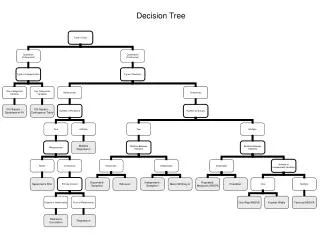
Definition • Decision tree is a classifier in the form of a tree structure • Decision node: specifies a test on a single attribute • Leaf node: indicates the value of the target attribute • Arc/edge: split of one attribute • Path: a disjunction of test to make the final decision • Decision trees classify instances or examples by starting at the root of the tree and moving through it until a leaf node.
Illustration (1) Which to start? (root) (2) Which node to proceed? (3) When to stop/ come to conclusion?
Random split • The tree can grow huge • These trees are hard to understand. • Larger trees are typically less accurate than smaller trees.
Principled Criterion • Selection of an attribute to test at each node - choosing the most useful attribute for classifying examples. • information gain • measures how well a given attribute separates the training examples according to their target classification • This measure is used to select among the candidate attributes at each step while growing the tree
Entropy • A measure of homogeneity of the set of examples. • Given a set S of positive and negative examples of some target concept (a 2-class problem), the entropy of set S relative to this binary classification is E(S) = - p(P)log2 p(P) – p(N)log2 p(N)
Suppose S has 25 examples, 15 positive and 10 negatives [15+, 10-]. Then the entropy of S relative to this classification is E(S)=-(15/25) log2(15/25) - (10/25) log2 (10/25)
Some Intuitions • The entropy is 0 if the outcome is ``certain’’. • The entropy is maximum if we have no knowledge of the system (or any outcome is equally possible). Entropy of a 2-class problem with regard to the portion of one of the two groups
Information Gain • Information gain measures the expected reduction in entropy, or uncertainty. • Values(A) is the set of all possible values for attribute A, and Sv the subset of S for which attribute A has value v Sv = {s in S | A(s) = v}. • the first term in the equation for Gain is just the entropy of the original collection S • the second term is the expected value of the entropy after S is partitioned using attribute A
It is simply the expected reduction in entropy caused by partitioning the examples according to this attribute. • It is the number of bits saved when encoding the target value of an arbitrary member of S, by knowing the value of attribute A.
Examples • Before partitioning, the entropy is • H(10/20, 10/20) = - 10/20 log(10/20) - 10/20 log(10/20) = 1 • Using the ``where’’ attribute, divide into 2 subsets • Entropy of the first set H(home) = - 6/12 log(6/12) - 6/12 log(6/12) = 1 • Entropy of the second set H(away) = - 4/8 log(6/8) - 4/8 log(4/8) = 1 • Expected entropy after partitioning • 12/20 * H(home) + 8/20 * H(away) = 1
Using the ``when’’ attribute, divide into 3 subsets • Entropy of the first set H(5pm) = - 1/4 log(1/4) - 3/4 log(3/4); • Entropy of the second set H(7pm) = - 9/12 log(9/12) - 3/12 log(3/12); • Entropy of the second set H(9pm) = - 0/4 log(0/4) - 4/4 log(4/4) = 0 • Expected entropy after partitioning • 4/20 * H(1/4, 3/4) + 12/20 * H(9/12, 3/12) + 4/20 * H(0/4, 4/4) = 0.65 • Information gain 1-0.65 = 0.35
Decision • Knowing the ``when’’ attribute values provides larger information gain than ``where’’. • Therefore the ``when’’ attribute should be chosen for testing prior to the ``where’’ attribute. • Similarly, we can compute the information gain for other attributes. • At each node, choose the attribute with the largest information gain.
Stopping rule • Every attribute has already been included along this path through the tree, or • The training examples associated with this leaf node all have the same target attribute value (i.e., their entropy is zero). Demo
Continuous Attribute? • Each non-leaf node is a test, its edge partitioning the attribute into subsets (easy for discrete attribute). • For continuous attribute • Partition the continuous value of attribute A into a discrete set of intervals • Create a new boolean attribute Ac , looking for a threshold c, How to choose c ?
Evaluation • Training accuracy • How many training instances can be correctly classify based on the available data? • Is high when the tree is deep/large, or when there is less confliction in the training instances. • however, higher training accuracy does not mean good generalization • Testing accuracy • Given a number of new instances, how many of them can we correctly classify? • Cross validation
Strengths • can generate understandable rules • perform classification without much computation • can handle continuous and categorical variables • provide a clear indication of which fields are most important for prediction or classification
Weakness • Not suitable for prediction of continuous attribute. • Perform poorly with many class and small data. • Computationally expensive to train. • At each node, each candidate splitting field must be sorted before its best split can be found. • In some algorithms, combinations of fields are used and a search must be made for optimal combining weights. • Pruning algorithms can also be expensive since many candidate sub-trees must be formed and compared. • Do not treat well non-rectangular regions.