Graphs and basic search algorithms
Graphs and basic search algorithms. Motivation Definitions and properties Representation Breadth-First Search Depth-First Search Chapter 22 in the textbook (pp 221—252). Motivation. Many situations can be described as a binary relation between objects: Web pages and their accessibility

Graphs and basic search algorithms
E N D
Presentation Transcript
Graphs and basic search algorithms • Motivation • Definitions and properties • Representation • Breadth-First Search • Depth-First Search Chapter 22 in the textbook (pp 221—252).
Motivation • Many situations can be described as a binary relation between objects: • Web pages and their accessibility • Roadmaps and plans • Transition diagrams • A graph is an abstract structure that describes a binary relation between elements. It is a generalization of a tree. • Many problems can be reduced to solving graph problems: shortest path, connected components, minimum spanning tree, etc.
Example: finding your way in the Metro • Stations are vertices (nodes) • Line segments are edges. • Shortest path = shortest distance, time. • Reachable stations. finish start
Graph (גרפים): definition • A graph G = (V,E) is a pair, where V = {v1, .. vn} is the vertex set (nodes) and E = {e1, .. em} is the edge set. An edge ek = (vi,vj) connects(is incident to)two vertices viand vjof V. • Edges can be undirected or directed (unordered or odered): eij:vi— vj oreij:vi—> vj • The graph G is finite when |V| and |E| are finite. • The size of graph G is |G| = |V| + |E|.
Directed graph Undirected graph 1 2 3 1 2 3 4 5 6 4 5 6 Graphs: examples Let V = {1,2,3,4,5,6}
2 The cost of a path is the sum of the costs of its edges: 1 2 3 5 4 1 8 4 5 6 Weighted graphs • A weighted graph is graph in which edges have weights (costs) c(vi, vj)> 0. • A graph is a weighted graph in which all costs are 1. Two vertices with no edge (path) between them can be thought of having an edge (path) with weight ∞. 6 7
Directed graphs • In a directed graph, we say that an edge e = (u,v) leaves u and enters v (v is adjacent, a neighbor of u). • Self-loops are allowed: an edge can leave and enter u. • The in-degreedin(v) of a vertex v is the number of edges entering v. The out-degreedout(v) of a vertex v is the number of edges leaving v. Σdin(vi) = Σdout(vi) • A path from u to v in G = (V,E) of length k is a sequence of vertices <u = v0,v1,…, vk = v> such that for every i in [1,…,k] the pair (vi–1,vi) is in E.
Undirected graphs • In an undirected graph, we say that an edge e = (u,v) is incident on u and v. • Undirected graphs have no self-loops. • Incidency is a symmetric relation: if e = (u,v) then u is a neighbor of vandv is a neighbor of u. • The degree of a vertex d(v) is the total number of edges incident on v. Σd(vi) = 2|E|. • Path: as for directed graphs.
Graphs terminology • A cycle (circuit) is a path from a vertex to itself of length ≥ 1 • A connected graph is an undirected graph in which there is a path between any two vertices (every vertex is reachable from every other vertex). • A strongly-connected graph is a directed graph in which for any two vertices u and v there is a directed path from u to v and from v to u. • A graph G’= (V’,E’) is a sub-graph of G = (V,E), G’ G when V’ V and E’ E. • The (strongly) connected componentsG1, G2, … of a graph G are the largest (strongly) connected sub-graphs of G.
Size of graphs • There are at most |E| = O(|V|2) edges in a graph. Proof: each node can be in at most |V| edges. A graph in which |E| = |V|2 is called a clique. • There are at least |E| |V|–1 edges in a connected graph. Proof: By induction on the size of V. • A graph is planar if it can be drawn in the plane with no two edges crossing. In a planar graph, |E| = O(|V|). The smallest non-planar graph has 5 vertices.
Trees and graphs • A tree is a connected graph with no cycles. • A tree has |E| =|V|–1 edges. • The following four conditions are equivalent: 1. G is a tree. 2. G has no cycles; adding a new edge forms a cycle. 3. G is connected; deleting any edge destroys its connectivity. 4. G has no self-loops and there is a path between any two vertices. • Similar definitions for a directed tree.
Graphs representation Two standard ways of representing graphs: • Adjacency list: for each vertex v there is a linked list Lvof its neighbors in the graph. Size of the representation: (|V|+|E|). • Adjacency matrix: a |V| ×|V| matrix in which an edge e = (u,v) is represented by a non-zero (u,v) entry. Size of the representation: (|V|2). Adjacency lists are better for sparse graphs. Adjacency matrices are better for dense graphs.
V Li 1 5 2 2 1 5 3 6 null 4 5 1 2 3 2 1 6 3 4 5 6 Example: adjacency list representation V ={1,2,3,4,5,6} E = {(1,2),(1,5),(2,5),(3,6)}
A 1 2 3 4 5 6 1 1 1 1 1 2 1 3 4 1 2 3 1 1 5 1 6 4 5 6 Example: adjacency matrix representation V ={1,2,3,4,5,6} E = {(1,2),(1,5),(2,5),(3,6)} For undirected graphs, A = AT
Graph problems and algorithms • Graph traversal algorithms • Breath-First Search (BFS) • Depth-First Search (DFS) • Minimum spanning trees (MST) • Shortest-path algorithms • Single path • Single source shortest path • All-pairs shortest path • Strongly connected components • Other problems: planarity testing, graph isomorphism
Shortest path problems There are three main types of shortest path problems: • Single path: given two vertices, s and t, find the shortest path from s to t and its length (distance). • Single source: given a vertex s, find the shortest paths to all other vertices. • All pairs: find the shortest path from all pairs of vertices (s, t). We will concentrate on the single source problem since 1. ends up solving this problem anyway, and 3. can be solved by applying 2. |V| times.
Intuition: how to search a graph • Start at the vertex s and label its level at 0. • If t is a neighbor of s, stop. Otherwise, mark the neighbors of s as having level 1. • If t is a neighbor of a vertex at level i, stop. Otherwise, mark the neighbors of vertices at level i as having level i+1. • When t is found, trace the path back by going to vertices at level i, i –1, i –2, …0. • The graph becomes in effect a shortest-path neighbor tree!
a b c s t d e f Example: a graph search problem...
level 0 1 2 3 4 5 6 a d a b c b d a e s t d e f … becomes a tree search problem s c e e b b f d f b f c e a c t t c t f t
How is the tree searched? The tree can be searched in two ways: • Breadth: search all vertices at level i before moving to level i+1 Breadth-First Search (BFS). • Depth: follow the vertex adjacencies, searching a node at each level i and backing up for alternative neighbor choices Depth-First Search (DFS).
level 0 1 2 3 4 a b c s t d e f Breadth-first search s a d b e c f t
a b c s t d e f Depth-first search s a b c e f t
The BFS algorithm: overview • Search the graph by successive levels (expansion wave) starting at s. • Distinguish between three types of vertices: • visited: the vertex and all its neighbors have been visited. • current: the vertex is at the frontier of the wave. • not_visited: the vertex has not been reached yet. • Keep three additional fields per vertex: • the type of vertex label[u]: visited, current, not_visited • the distance from the source s, dist[u] • the predecessor of u in the search tree, π[u]. • The current vertices are stored in a queue Q.
The BFS algorithm BFS(G, s) label[s] current; dist[s] = 0; π[s] = null for all vertices u in V – {s} do label[u] not_visited; dist[u] = ∞; π[u] = null EnQueue(Q,s) whileQ is not emptydo u DeQueue(Q) for each v that is a neighbor ofu do iflabel[v] = not_visitedthenlabel[v] current dist[v] dist[u] + 1; π[v] u EnQueue(Q,v) label[u] visited
Breath-first tree a b c s t d e f Example: BFS algorithm 1 2 3 0 4 1 2 3
BFS characteristics • Q contains only current vertices. • Once a vertex becomes current or visited, it is never labeled again not_visited. • Once all the neighbors of a current vertex have been considered, the vertex becomes visited. • The algorithm can be easily modified to stop when a target t is found, or report that no path exists. • The BSF algorithm builds a predecessor sub-graph, which is a breath-first tree: Gπ = (Vπ,Eπ)Vπ= {vV: π[v] ≠ null}{s} and Eπ= {(π[v],v), vV –{s}}
Complexity of BFS • The algorithm removes each vertex from the queue only once. There are thus |V| DeQueue operations. • For each vertex, the algorithm goes over all its neighbors and performs a constant number of operations. The amount of work per vertex in the if part of the while loop is a constant times the number of outgoing edges. • The total number of operations (if part) for all vertices is a constant times the total number of edges |E|. • Overall: O(|V|) + O(|E|) = O(|V|+|E|), at most O(|V|2)
The DFS algorithm: overview (1) • Search the graph starting at s and proceed as deep as possible (expansion path) until no unexplored vertices remain. Then go back to the previous vertex and choose the next unvisited neighbor (backtracking). If any undiscovered vertices remain, select one of them as the source and repeat the process. • Note that the result is a forest of depth-first trees: Gπ = (V,Eπ) Eπ= {(π[v],v), vV and π[v] ≠ null} where π[v] is the predecessor of v in the search tree • As for BFS, there are three three types of vertices: visited, current, and not_visited.
The DFS algorithm: overview (2) • Two additional fields holding timestamps. • d[u]: timestamp when u is first discovered (u becomes current). • f [u]: timestamp when the neighbors of u have all been explored (u becomes visited). • Timestamps are integers between1 and 2|V|, and for every vertex u, d[u] < f [u]. • Backtracking is implemented with recursion.
The DFS algorithm DFS(G, s) label[s] current; dist[s] = 0; π[s] = null; time 0. for each vertex u in do iflabel[u] =not_visited thenDFS-Visit(u) DFS-Visit(u) label[u] = current; time time +1; d[u] time for each v that is a neighbor ofu do iflabel[v] = not_visitedthen π[v] u; DFS-Visit(v) label[u] visited f [u] time time + 1
Depth-first tree a b c s t d e f Example: DFS algorithm 2/15 3/14 4/5 1/16 Time: discovery/finish 8/9 11/12 6/13 7/10
DFS characteristics • The depth-first forest that results from DFS depends on the order in which the neighbors of a vertex are selected to deepen the search. • The DFS program be easily modified to search only from start vertex s, and to find the shortest path from s to t. • Instead of recursion, a LIFO queue can be used (instead of FIFO for BFS). • The history of discovery and finish times, d[v] and f [v], has a parenthesis structure.
DFS: parenthesis structure (1) 2/15 3/14 4/5 a b c Discovery:open ( push Finish:close ) pop 1/16 s 8/9 t d e f 11/12 6/13 7/10 (s (a (b (c c) (e (f (t t) f) (d d) e) b) a) s) 1 2 3 4 5 6 7 8 910 11 121314 15 16
DFS: parenthesis structure (2) (s (a (b (c c) (e (f (t t) f) (d d) e) b) a) s) 1 2 3 4 5 6 7 8 910 11 121314 15 16 (ss) 1 (aa)16 2 (bb)15 3 (c c) (ee) 14 456 (ff) (d d) 13 7 (t t) 101112 8 9
Complexity of DFS • The algorithm visits every node vV Θ(|V|) • For each vertex, the algorithm goes over all its neighbors and performs a constant number of operations. • Overall, DFS-Visit is called only once for each v in V, since the first thing that the procedure does it label v as current. • In DFS-Visit, the recursive call is made for at most the number of edges incident to v: ΣvV|neighbors[v]| = Θ(|E|) • Overall:Θ(|V|) + Θ(|E|) = Θ(|V|+|E|), at most Θ(|V|2) • Same complexity as BFS!
Classification of edges Edges in the depth-first forest Gπ = (V,Eπ) and Eπ= {(π[v],v), vV and π[v] ≠ null} can be classified into four categories: • Tree edges: depth-first forest edges in Eπ • Back edges: edges (u,v) connecting a vertex u to an ancestor v in a depth-first tree (includes self-loops) • Forward edges: non-tree edges (u,v) connecting a vertex u to a descendant v in a depth-first tree. • Cross edges: all other edges. Go between vertices in the same depth-first tree without an ancestor relation between them.
b f e d g Tree edges a s Back edges Forward edges Cross edges Example: DFS edge classification
Summary: Graphs, BFS, and DFS • A graph is a useful representation for binary relations between elements. Many problems can be modeled as graphs, and solved with graph algorithms. • Two ways of finding a path between a starting vertex s and all other vertices of a graph: • Breath-First Search (BFS): search all vertices at level i before moving to level i+1. • Depth-First search(DFS): follow vertex adjacencies, one vertex at each level i and backtracking for alternative neighbor choices. • Complexity: linear in the size of the graph: Θ(|V|+|E|)
Minumum spanning trees • Motivation • Properties of minimum spanning trees • Kruskal’s algorithm • Prim’s algorithm Chapter 23 in the textbook (pp 561—579).
Motivation • Given a set of nodes and possible connections with weights between them, find the subset of connections that connects all the nodes and whose sum of weights is the smallest. • Examples: • telephone switching network • electronic board wiring • The nodes and subset of connections form a tree! • This tree is called the Minimum Spanning Tree (MST – (עץ פורש מינימום
8 7 b c d 11 a i e h g f Cost: 51 Example: spanning tree 4 9 2 14 4 7 6 8 10 1 2
7 8 4 9 b c d 2 11 a i e 14 4 7 6 h g f 8 10 1 2 Cost: 37 Example: minimum spanning tree
Spanning trees • Definition: Let G=(V,E) be a weighted connected undirected graph. A spanning tree of G is a subset T E of edges, such that the sub-graph G’=(V,T) is connected and acyclic. • Theminimum spanning tree (MST) is a spanning tree that minimizes the sum:
Generic MST algorithm Greedy strategy: grow the minimum spanning tree one edge at a time, making sure that the added edge preserves the tree structure and the minimality condition add “safe” edges incrementally. Generic-MST(G=(V,E)) T = ; while (T is not a spanning tree of G) do choose a safe edge e=(u,v) E T = T {e} return T
T Properties of MST (1) • Question: how to find safe edges efficiently? • Theorem 1: Let and e=(u,v) be a minimum weight edge with one endpoint in U and the other in V–U. Then there exists a minimum spanning tree T such that e is in T. V U V–U
8 7 b c d 11 a i e h g f Properties of MST (2) U cut V–U 4 9 2 14 4 7 6 8 10 1 2
Properties of MST (2) Proof: Let T be an MST. If e is not in T, add e to T. Because T is a tree, the addition of e creates a cycle which contains e and at least one more edge e’=(u’,v’), where u’U and v’ V–U. Clearly, w(e) ≤w(e’) since e is of minimum weight among the edges connecting U and V–U. We can thus delete e’ from T. The resulting T’ = T – {e’}{e} is a tree whose weight is less or equal than that of T: w(T’) ≤w(T).
T Properties of MST (3) Theorem 2: Let G=(V,E) be a connected undirected graph and A a subset of E included in a minimum spanning tree T for G. Let (U, V–U) be a cut that respects A (no edge of A crosses the cut), and let e=(u,v) be a minimum weight edge crossing (U, V–U). Then e is safe for A. V U V–U A = T E’ cut
Properties of MST (4) Proof: Define an edge e to be a light edge crossing a cut if its weight is the minimum crossing the cut. Let T be an MST that includes A, and assume T does not contain the light edge e = (u,v) (if it does, e is safe). Construct another MST T’ that includes A {e}. The edge forms a cycle with edges on the path p from u to v in T. Since u and v are on opposite sides of the cut, there is at least one edge e’ = (x,y) in T on the path p that also crosses the cut. The edge e’ is not in A because the cut respects A. Since e’ is on the unique path from u to v in T, removing it breaks T into two components.
Properties of MST (5) Adding e = (u,v) reconnects the two components to form a new spanning tree: T’ = T –{e’} {e} We now show that T’ is an MST. Since e = (u,v) is a light edge crossing (U, V–U) and e’ = (x,y) also crosses this cut, w(u,v) ≤ w(x,y). Thus: w(T’) = w(T) – w(u,v) + w(x,y) ≤ w(T) Since T is an MST and w(T’) ≤ w(T), then w(T’) =w(T) and T’ is also an MST.