Download
1 / 52
520 likes | 539 Vues
Learn how to derive camera coordinate systems for accurate projection in 3D views and simplify computations for better visualization.

E N D
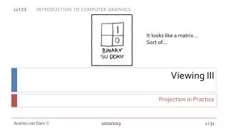
Viewing III Projection in Practice 10/10/2019
Arbitrary 3D views • view volumes/frusta specified by placement & shape • Placement: • Position(a point) • lookand upvectors • Shape: • Horizontal and vertical view angles (for a perspective v.v.) • Front and back clipping planes* • Note that camera coordinate system (u, v, w) is defined in the world (x, y, z) coordinate system • Roadmap: first derive (u, v, w) coordinate system from camera specs, then “normalize” that coordinate system so camera is at the origin looking down the negative z axis, to simplify computation • Note: The book refers to up as vup, while Viewing II uses Up. They all refer to the same vector. *conventionally called near and far clipping planes, although actually they are rectangles in the plane (because they have bounds) 10/10/2019
Finding u, v, and w from Position, look, and up (1/5) • We want the u, v, w orthonormal camera coordinate system axes to have the following properties: • Our arbitrary lookvector will lie along the negative w-axis • The v-axis will be defined by the vector perpendicular to look, and will liein the plane defined bylookand up • Theu-axis will be mutually perpendicular to the v- and w-axes, and will form a right-handed coordinate system • First find w fromlook, then find vfrom up and w, then find u as a normal to the wv-plane 10/10/2019
Finding u, v, and w from Position, look, and up (2/5) • Finding w is easy. look in the canonical volume lies on –w, so wis a normalized vector pointing in the direction opposite to look 10/10/2019
Finding u, v, and w from Position, look, and up (3/5) • Findingv • Problem: we have to find a unit vector v that is perpendicular to the unit vector w in the look-up plane • Solution: subtract the w component of the up vector to get v’ and normalize. To get w component w’ of up, project up onto w: Projection of up onto w, because w is a unit vector w Looking directly at wv-plane 10/10/2019
Finding u, v, and w from Position, look, and up (4/5) • Findingu • We can use the cross-product, but which? Both w × v and v × w are perpendicular to the plane, but they go in opposite directions. • Answer: cross-products are “right-handed,” so use v × w to create a right-handed coordinate frame • As a reminder, the cross product of two vectors a and b is: 10/10/2019
Finding u, v, and w from Position, look, and up (5/5) • To Summarize: • Now that we have defined our camera coordinate system, how do we calculate projection? 10/10/2019
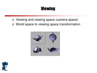
The Canonical View Volume • How to take contents of an arbitrary view volume and project them to a 2D surface? • arbitrary view volume is too complex… • Reduce it to a simpler problem! The canonical view volume! • Easiest case: parallel view volume (aka standard view volume) • Specific orientation, position, height and width that simplify clipping, VSD (visible surface determination) and projecting • Transform complex view volume and all objects in volume to the canonical volume (normalizing transformation) and then project contents onto normalized view plane • This maintains geometric relationships between camera and objects, but computationally, we only transform objects • Don’t confuse with animation where camera may move relative to objects! Normalization applies to an arbitrary camera view at a given instant Image credit: http://www.codeguru.com/cpp/misc/misc/math/article.php/c10123__2/ 10/10/2019
The Canonical Parallel View Volume • Sits at the origin: • Center of near clipping plane = (0,0,0) • Looks along negative z-axis (corresponds to scene • behind the “looking glass”) • look vector = (0,0,-1) • Oriented upright (along y-axis): • v vector = (0,1,0) • Viewing window bounds normalized: • -1 to 1 in x and y directions • Near and far clipping planes: • Near at z = 0 plane (‘front’ in diagram) • Far at z = -1 plane (‘back’ in diagram) • Note: making our view plane bounds -1 to 1 makes the arithmetic easier 10/10/2019
The Normalizing Transformation • Goal: transform arbitrary view and scene to canonical view volume, maintaining relationship between view volume and scene, then render • For a parallel view volume, need only translation to the origin, rotation to align u, v, w with x, y, z, and scaling to size • The composite transformation is a 4x4 homogeneous matrix called the normalizing transformation (the inverse is called the viewing transformation and turns a canonical view volume into an arbitrary one) • Note: the scene resulting from normalization will not appear any different from the original – every vertex is transformed in the same way. The goal is to simplify calculations on our view volume, not change what we see • Normalizing demo: http://cs.brown.edu/courses/cs123/demos/camera/ Y Remember our camera is just an abstract model; The normalizing matrix needs to be applied to every vertex in our scene to simulate this transformation. X Z Pn P0 10/10/2019
View Volume Translation • Our goal is to send the u,v,w axes of camera’s coordinate system to coincide with the x, y, z axes of the world coordinate system • Start by moving camera so the center of the near clipping plane is at the origin • Given camera position P0defining the origin of the uvw-coordinate system, w axis, and the distances to the near and far clipping planes, the center of the near clipping plane is located at Pn = P0 - near*w • This matrix translates all world points and camera so that Pn is at the origin 10/10/2019
View Volume Rotation (1/3) • Rotating the camera/scene can’t be done easily by inspection • Our camera is now at the origin; we need to align the u, v, w axes with the x, y, z axes • This can be done by separate rotations about principle axes (as discussed in the Transformations lecture), but we are going to use a more direct (and simpler) approach • Let’s leave out the homogeneous coordinate for now • Consider the standard unit vectors for the XYZ world coordinate system: • We need to rotate u into e1 and v into e2 and w into e3 • Need to find some composite matrix Rrot such that: • Rrotu = e1Rrotv = e2Rrotw = e3 10/10/2019
View Volume Rotation (2/3) • How do we find Rrot? Let’s manipulate the equations to make the problem easier and first find Rrot-1. After multiplying on both sides by Rrot-1, we get: • u = Rrot-1e1 • v = Rrot-1e2 • w = Rrot-1e3 • Recall from the Transformations lecture that this means exactly that u is the first column of Rrot-1, v is the second column, and w is the third column • Therefore, we have 10/10/2019
View Volume Rotation (3/3) • Now we need to invert Rrot-1 • The axes u, v, and w are orthogonal, and since they are unit vectors, they are also orthonormal • This makes Rrot-1 an orthonormal matrix (its columns are orthonormal vectors). This means that its inverse is just its transpose (we proved this in the Transformations lecture!) • Therefore, non-homogeneous coordinates: Homogeneous form 10/10/2019
Scaling the View Volume • Now we have a view volume sitting at the origin, oriented upright with look pointing down the –z axis • The size of our volume still does not meet our specifications • We want the (x, y) bounds to be at -1 and 1 and we want the far clipping plane to be at z = -1 • Given width, height, and far clipping plane distance, far, all positive magnitudes, our scaling matrix Sxyz is: • Now all vertices post-clipping are bounded in between planes x = (-1, 1), y = (-1, 1), z = (0, -1) 10/10/2019
The Normalizing Transformation (parallel) and Re-Homogenization • Have a complete transformation from arbitrary parallel view volume to canonical parallel view volume • Use position, look, and up to calculate u, v, w local camera coordinate system • First translate Pn(center of near plane) to origin using translation matrix Ttrans • Then align u, v, w axes with x, y, z axes using rotation matrix Rrot • Finally, scale view volume using scaling matrix Sxyz • Composite normalizing transformation is SxyzRrotTtrans • Since each individual transformation results in w = 1, no division by w to re-homogenize is necessary! 10/10/2019
Notation • The book groups all of these three transformations together into one transformation matrix • For the parallel case, we will call it Morthogonal • For the perspective case, which we will get to next, it is called Mperspective • For ease of understanding, we split all three up but they can be represented more compactly by the following, where N is the 3x3 matrix representing rotations and scaling: 10/10/2019
Clipping Against the Parallel View Volume • Before returning to original goal of projecting scene onto view plane, how do we clip? • With arbitrary view volume, the testing to decide whether a vertex is in or out is done by solving simultaneous equations • With canonical view volume, clipping is much easier: after applying normalizing transformation to all vertices in scene, anything that falls outside the bounds of the planes x = (-1, 1), y = (-1, 1), and z = (0, -1) is clipped • First check whether bounding box is inside or outside (easy cases) and do clipping of primitives only if it intersects. Primitives that intersect view volume must be partially clipped. • Most graphics packages, e.g. OpenGL, do this step for you Note: Clipping edges that intersect the boundaries of view volume is another step explored in clipping lecture 10/10/2019
Projecting in the Normalized View Volume • So how do we project the scene in this normalized view volume onto the (x, y) plane, where the view plane is now located? (view plane can be anywhere, having it at the origin makes arithmetic easy) • To project a point (x, y, z) onto the (x, y) plane, just get rid of the z coordinate! We can use the following matrix: • Most graphics packages also handle this step for you 10/10/2019
Next: The Perspective View Volume • Need to find a transformation to turn an arbitrary perspective view volume into a canonical (unit) perspective view volume Canonical view volume (frustum): Far clipping plane (-1,1,-1) z = -1 (1,-1,-1) Near clipping plane 10/10/2019
Properties of the Canonical Perspective View Volume • Sits at origin: • Position = (0, 0, 0) • Looks along negative z-axis: • look vector = (0, 0, -1) • Oriented upright • v vector = (0, 1, 0) • Near and far clipping planes • Near plane at z = c = -near/far (we’ll explain this; • near and far are positive distances) • Far plane at z = -1 • Far clipping plane bounds: • (x, y) from -1 to 1 • Note: the perspective canonical view volume is just like the parallel one except that the “film/projection” plane is more ambiguous here; we’ll finesse the question by transforming the normalized frustum into the normalized parallel view volume before clipping and projection! Far clipping plane z = -1 (-1,1,-1) (1,-1,-1) Near clipping plane 10/10/2019
Translation and Rotation • For our normalizing transformation, the first two steps are the same • The translation matrix Ttrans is even easier to calculate this time, since we are given the point P0 to translate to origin. We use the same matrix Rrot to align camera axes: • Our current situation: y z x 10/10/2019
Scaling • For perspective view volumes, scaling is more complicated and requires some trigonometry • Easy to scale parallel view volume if we know width and height • Our definition of frustum, however, doesn’t give these two values, only θw and θh • We need a scaling transformation Sxyz that: • Finds width and height of far clipping plane based on width angle θw, height angle θh , and distance far to the far clipping plane • Scales frustum based on these dimensions to move far clipping plane to z = -1 and to make corners of its cross section move to ±1 in both x and y • Scaling position of far clipping plane to z = -1 remains same as parallel case, since we are still given far; however, unlike parallel case, near plane not mapped to z = 0 10/10/2019
Scaling the Perspective View Volume (1/4) • Top-down view (looking down the y axis) of the perspective view volume with arbitrary rectangular cross-section: • Goal: scale the original volume so the solid arrows are transformed to the dotted arrows and the far plane’s cross-section is squared up, with corner vertices at (±1, ±1, -1) • i.e., scale the original (solid) far plane cross-section F so it lines up with the canonical (dotted) far plane cross-section F’ at z = -1 • First, scale along z direction • Want to scale so far plane lies at z = -1 • Far plane originally lies at z = -far • Multiply by 1/far, since –far/far = -1 • So, Scalez = 1/far 10/10/2019
Scaling the Perspective View Volume (2/4) • Next, scale along x direction • Use the same trick: divide by size of volume along the x-axis • How long is the (far) side of the volume along x? Find out using trig… • Start with the original volume • Cut angle in half along the z-axis far far θw /2 θw z z θw /2 x x 10/10/2019
Scaling the Perspective View Volume (3/4) • Consider just the top triangle • Note that L equals the x-coordinate of a corner of the perspective view volume’s cross-section at far. Ultimately want to scale by 1/L to make L → 1 • Thus 10/10/2019
Scaling the Perspective View Volume (4/4) • Finally, scale along y direction • Use the same trig as in xdirection, but use the height angle instead of the width angle: • Together with the x- and z-scale factors, we have: 10/10/2019
The Normalizing Transformation (perspective) • Our current perspective transformation takes on the same form as the parallel case: • Use position, look, and up to calculate u, v, w local camera coordinate system • Takes the camera’s position and moves it to the world origin • Orients the camera to look down the –z axis • Scales the view volume so that the far clipping plane lies on z=-1 plane, with corners are at (±1, ±1, -1) • Multiplying any point P by this matrix, the resulting point P’ will be the normalized version • The projected scene will still look the same as if we had projected it using the arbitrary frustum, since same composite is applied to all objects in the scene, leaving the camera-scene relationship invariant. 10/10/2019
Notation • We can represent this composite matrix as Mperspective by the following: • Here, N is the 3x3 matrix representing rotations and scaling 10/10/2019
Perspective and Projection • However, projecting even a perspective view volume onto a 2D plane is more difficult than it was in the parallel case since we’d have to consider each projector thru a vertex • Again: reduce it to a simpler problem! • The final step of our normalizing transformation – transforming the perspective view volume into a parallel one – will preserve relative depth, which is crucial for Visible Surface Determination, i.e., the occlusion problem • Simplifies not only projection (just leave off z component), but also clipping and visible surface determination – only have to compare z-values (z-buffer algorithm) • Performs crucial perspective foreshortening step • Think of this non-affine perspective-to-parallel transformation pp as the unhinging transformation, represented by matrix Mpp Note: near rectangle has been moved to z=0, in the xy plane, with its center at the origin 10/10/2019
Effect of Perspective Transformation on Near Plane (1/2) • Previously we transformed perspective view volume to canonical position, orientation, and size • We’ll see in a few slides that Mpp leaves the far clip plane at z=-1, and its cross-section undistorted, with corners at ±1; all other cross-sections will be perspectively foreshortened • Let’s first look how Mperspectivemaps a particular point on the original near clipping plane lying on look (we denote the normalized look vector by look’ ): • It gets moved to a new location: • On the negative z-axis, say: c is a negative number between -1 and 0 10/10/2019
Effect of Perspective Transformation on Near Plane (2/2) • What is the value of c? Let’s trace through the steps. • P0 first gets moved to the origin • The point Pn is then distortion-free (rigid-body) rotated to –near*z • The xyscaling has no effect, and the far scaling moves Pn to (-near/far)*z, so c= -near/far 10/10/2019
Unhinging Canonical Frustum to Be a Parallel View Volume(1/4) • Note from figure that far clipping plane cross-section is already in right position with right size • Near clipping plane at –near/far should transform to the plane z=0 z = -near/far -z z = -1 10/10/2019
Unhinging Canonical Frustum to Be a Parallel View Volume (2/4) • The derivation of our unhinging transformation is complex. Instead, we will give you the matrix and show that it works by example (“proof by vigorous assertion/demonstration") • Our unhinging transformation matrix to map perspective to parallel, Mpp • Remember, c = -near/far 10/10/2019
Unhinging View Volume to Become a Parallel View Volume(3/4) • Our perspective transformation does the following: • Sends all points on the z= -1 far clipping plane to themselves • Check top-left (-1, 1, -1, 1) and bottom-right (1, -1, -1, 1) corners to see they don’t change • Sends all points on the z = c near clipping plane onto the z = 0 plane • Note that the corners of the square cross section of the near clipping plane in the frustum are (±c,±c,c,1) because it is a rectangular (square) pyramid w/ 45° planes • Check to see that top-left corner (c,-c,c,1) gets sent to (-1, 1, 0, 1) and that bottom-right corner (-c,c,c,1) gets sent to (1, -1, 0, 1) • Let’s try c = -1/2 10/10/2019
Unhinging View Volume to Become a Parallel View Volume(4/4) y (-1,1,-1) (c,-c, c) = (-1/2, 1/2, -1/2) z (-c,c,c) (1,-1,-1) x (-1,1,-1) Don’t forget to homogenize! Homogenization with a w≠1 does the perspective foreshortening! (-1,1,0) (1,-1,-1) (1,-1,0) Note: Diagram is deceptive because a parallel projection is used in illustration, but center of front clipping plane is at origin 10/10/2019
Perspective Foreshortening Affects x, y, and z Values • Let’s apply Mpp to an arbitrary (x, y, z) point: • Note x and y are both divided by z, but z value is fractional - the closer it is to 0 (the CoP/eye/camera), the larger the x and y values scale up • But then we clip – if x or y exceed 1, they’ll be clipped, hence the utility of the near plane which prevents such unnecessary clipping and obscuration of rest of scene • We’ll look at the effects on z (z-compression) on slide 44-46 10/10/2019
Practical Considerations: z-buffer for Visible Surface Determination • Cross-sections inside view volume are scaled up the closer they are to near plane to produce perspective foreshortening, and z values decrease, but relative z-distances and therefore order are preserved • Depth testing using a z-buffer (aka depth-buffer) that stores normalized z-values of points compares a point on a polygon being rendered to one already stored at the corresponding pixel location – only relative distance matters • z-buffer uses alternate form of Mpp that does the same unhinging as the original but negates the z-term to make the volume point down the positive z-axis (use this one in camtrans lab, since we use a z-buffer) • The post-clipping range for these z-values is [0.0,1.0], where 0.0 corresponds to the near plane, and 1.0 to far 10/10/2019
Why Perspective Transformation Works (1/2) • Take an intuitive approach to see this • The closer the object is to the near clipping plane, the more it is enlarged during the unhinging step • Thus, closer objects are larger and farther away objects are smaller, as expected • Another way to see it is to use parallel lines • Draw parallel lines in a perspective volume • When unhinge volume, lines fan out at near clipping plane • Result is converging lines, e.g., railroad track coinciding at vanishing point 10/10/2019
Why Perspective Transformation Works(2/2) • Yet another way to demonstrate how this works is to use occlusion (when elements in the scene are blocked by other elements) • Looking at top view of frustum, we see a square • Draw a line from eye point to left corner of square – all points behind this corner are obscured by the corner (i.e. we can’t draw a projector to a point behind the corner w/o hitting the corner first) • Now unhinge perspective and draw a line again to left corner - all points obscured before are still obscured and all points that were visible before are still visible 10/10/2019
The Normalizing Transformation (perspective) • We now have our final normalizing transformation; call it to convert an arbitrary perspective view volume into a canonical parallel view volume • Remember to homogenize points after you apply this transformation – does the perspective! • Clipping and depth testing have both been simplified by transformation (use simpler bounds checking and trivial z-value comparisons resp.) • Additionally, can now project points to viewing window easily since we’re using a parallel view volume: just omit z-coordinate! Avoids having to pick a film/projection plane • Then map contents to viewport using window-to-viewport mapping (windowing transformation) 10/10/2019
The Windowing Transformation (1/2) • The last step in our rendering process after projecting is to resize our clip rectangle on the view plane, i.e., the cross-section of the view volume, to match the dimensions of the viewport • To do this, we want to have a viewing/clipping window with its lower left corner at (0,0) and with width and height equal to those of the viewport • This can be done using the windowing transformation – derived on next slide 10/10/2019
The Windowing Transformation (2/2) (1, 1) • First translate viewing window by 1 in both the x and y directions to align with origin and then scale uniformly by ½ to get proper unit size: • Then scale viewing window by width and height of viewport to get our desired result • Finally, translate the viewing window to be located at the origin of the viewport (any part of the screen) • Can confirm this matches more general windowing transformation in Transformations lecture -- handled by most graphics packages 10/10/2019
Perspective Transform Causes z-Compression (1/3) • Points are moved and compressed towards the far clipping plane • Let’s look at the general case of transforming a point by the unhinging transformation: • First, note that x and y are both shrunk for z > 1 (perspective foreshortening increasing with increasing z) – corresponds to what we first saw with similar triangles explanation of perspective • Now focus on new z-term, called z’. This represents new depth of point along z-axis after normalization and homogenization • z’ = (c-z)/(z+zc), now let’s hold c constant and plug in some values for z • Let’s have near = 0.1, far = 1, so c = -0.1 • The following slide shows a graph of z’ dependent on z 10/10/2019
Perspective Transform Causes z-Compression (2/3) z z’ • We can see that the z-values of points are being moved and compressed towards z = -1 in our canonical view volume -- this compression is more noticeable for points originally closer to the far clipping plane • Play around with near and far clipping planes: observe that as you bring the near clipping plane closer to z=0, or extend the far clipping plane out more, the z-compression becomes more severe • This results in binning: even though for real Z points are separated, they are put in the same integer bin when they are close • In fact, if z-compression is too severe, z-buffer depth testing becomes inaccurate near the back of the view volume and rounding errors can cause objects to be rendered out of order, i.e., “bleeding through” aka “z-fighting” of pixels occurs (upcoming VSD lecture) • Let’s look at this algebraically… 10/10/2019
Perspective Transform Causes Z-Compression (3/3) • It might seem tempting to place the near clipping plane at z = 0 or place the far clipping plane very far away (maybe at z = ∞) • First note that the value of c = -near/far approaches 0 as either near approaches 0 or as far approaches ∞ • Applying this to our value of z’ = (c-z)/(z+zc), we substitute 0 for c to get z’ = -z/z = -1 • From this, we can see that points will cluster at z = -1 (the far clipping plane of our canonical view volume) and depth-buffering essentially fails 10/10/2019
Aside: Projection and Interpolation(1/3) • This converging of points at the far clipping plane also poses problems when trying to interpolate values, such as the color between points • Say for example we color the midpoint M between two vertices, AandB, in a scene as the average of the two colors of A and B (assume we’re looking at a polygon edge-on or just an edge of a tilted polygon) • Note that if we were just using a parallel view volume, it would be safe to just set the midpoint to the average and we’re done • Unfortunately, we can’t do this for perspective transformations: M is compressed towards clipping plane. It isn’t the actual midpoint anymore. • The color does not interpolate between the points linearly anymore - can’t just assign the new midpoint the average color. (3/5,-4/5) 10/10/2019
Aside: Projection and Interpolation(2/3) • However, while color Gdoes not interpolate linearly, G/w does, where w is the homogenous coordinate after being multiplied by our normalizing transformation, but before being homogenized • In our case w will always be -z • Knowing this, how can we find the color at this new midpoint? • When we transform A and B, we get two w values, wA and wB • We also know the values of GA and GB • If we interpolate linearly between GA / wAand GB / wB (which in this case is just taking the average), we will know the value for the new midpoint GM / wM • We can also find the average of 1 / wA and 1 / wB and to get 1 / wM by itself • Dividing by GM / wM by 1 / wM , we can get our new value of GM 10/10/2019
Aside: Projection and Interpolation(3/3) • Let’s make this slightly more general • Say we have a function f that represents a property of a point (we used color in our example) • The point P between points A and B to which we want to apply the function is (1-t)A + tB for some 0 ≤t ≤ 1. The scalar t represents the fraction of the way from point A to point B your point of interest is (in our example, t = 0.5) • Goal: Compute f(P). We know • 1 / wt = (1-t) / wa + t / wb • f(P) / wt = (1-t)f(A) / wa + tf(B) / wb • So to find the value of our function at the point specified by t we compute: • f(P) = ( f(P) / wt ) / ( 1 / wt) 10/10/2019
Proof by Example • Let’s revisit the setup from this image: • Say we want f(A) = 0, f(B) = 1, and thus f(M) = 0.5 • After unhinging transformation, the new midpoint, is 4/5 of the way from A’ to B’, which can be found with some algebra: • M’y = (1-t)A’y + tB’y • t = (M’y – A’y) / (B’y – A’y) = 4/5 • Like f(M), f(M’) should be 0.5. We check this below: • wa = 0.25 and wb= 1 • 1/wt = (1-0.8)*(1/0.25) + 0.8*(1/1) = 1.6 • f(P)/wt = (1-0.8)*(0/0.25) + 0.8*1/1 = 0.8 • f(M’) = (f(P)/wt) / (1/wt) = 0.5 (3/5,-4/5) 10/10/2019