Download
1 / 64
640 likes | 680 Vues
Understand stochastic processes, models, estimators, random variables, filters, and more. Learn probability, independence, and use in computer science. Evaluation methods include midterm, presentation, MATLAB assignment, attendance, and final exam.

E N D
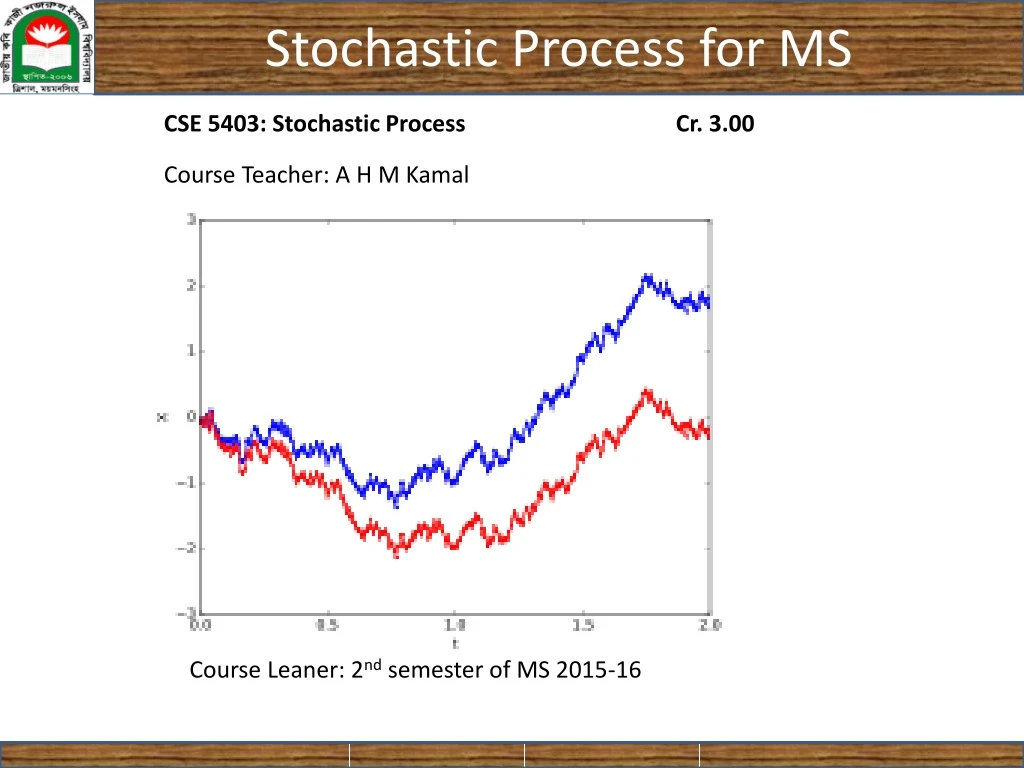
Stochastic Process for MS CSE 5403: Stochastic Process Cr. 3.00 Course Teacher: A H M Kamal Course Leaner: 2nd semester of MS 2015-16
Stochastic Process for MS A stochastic process is a probabilistic (non-deterministic) system that evolves with time via random changes to a collection of variables. A finite stochastic process consists of a finite number of stages in which the outcomes and associated probabilities at each stage depend on the outcomes and associated probabilities of the preceding stages. One type of finite stochastic process is called a Random Walk. A Random Walk process is "memoryless": the next state depends only on the current state and not on the sequence of events that preceded it. Input Outcome of Stage n Outcome and probabilities of Stage 1 Stage n Stage 1 Stage 2
Stochastic Process for MS Aim of the course: The object of this course is to lead to a good understanding of stochastic processes, their most commonly used models and their properties, as well as the derivation of some of the most commonly used estimators for such processes : Wiener and Kalman filters, predictors and smoothers At the end of this course, the students will be able to : -- Have a good understanding of and familiarity with random variables and stochastic processes ; -- Characterize and use stable processes and their spectral properties; -- Use the major estimators, and characterize their performances ; -- Synthetize predictors, filters and smoothers, in both Wiener or Kalman frameworks.
Stochastic Process for MS The course is subdivided into four parts/chapters: -- Probabilities, random variables, moments, change of variables. -- Stochastic processes, independence, stability, ergodicity, spectral representation, classical models of stochastic processes. -- Estimation (for random variables) : biais, variance, bounds, convergence, asymptotic properties, classical estimators. -- Estimation (for random processes) : filtering, prediction, smoothing, Wiener and Kalman estimators. However, we will learn few more topics in this course if we can manage time.
Stochastic Process for MS Is Stochastic Process useful for Computer Science Students? Stochastic processes underlie many ideas in statistics such as time series, markov chains, markov processes, bayesian estimation algorithms, etc. Thus, a study of stochastic processes will be useful in two ways: Enable you to develop models for situations of interest to you. Enable you to better understand the nuances of the statistical methodology that uses stochastic processes. The short answer probably is that all observable processes, which we may want to analyze with statistical tools, are stochastic processes, that is, they contain some element of randomness
Stochastic Process for MS CSE 5403: Stochastic Process Cr. 3.00 Course Teacher: A H M Kamal Evaluation Method: One mid Term 10% One presentation 10% Assignment to solve in MATLAB 10% Attendance 10% Final exam 60%
Stochastic Process for MS Why Randomness?
Stochastic Process for MS Randomness Key point: Outcomes 22} Adult suffrage Continuous 17 Office hours Days temperature Discrete Are you liking stochastic process course?
Stochastic Process for MS Randomness Key point: Outcomes Key point: Continuous and Discrete Sample Space
Stochastic Process for MS Why Randomness?
Stochastic Process for MS Event Often we are interested in a collection of related outcomes from a random experiment. An event is a subset of the sample space of a random experiment.
Stochastic Process for MS Probability
Stochastic Process for MS Probability
Stochastic Process for MS Probability
Stochastic Process for MS Probability
Stochastic Process for MS Probability Additional Rules: Two events: More events:
Stochastic Process for MS Probability Conditional Probability: When two events A, B are dependent it is important to know the probability that the event B will occur, given that A has already happened. We define this to be conditional probability, denoted by P(B|A).
Stochastic Process for MS Probability Conditional Probability: When two events A, B are dependent it is important to know the probability that the event B will occur, given that A has already happened. We define this to be conditional probability, denoted by P(B|A). Multiplication rule:
Stochastic Process for MS Probability Total Probability: Total Probability of B: As A and A’are mutually exclusive:
Stochastic Process for MS Probability Total Probability:
Stochastic Process for MS Probability Total Probability:
Stochastic Process for MS Probability: Independence
Stochastic Process for MS Probability: Independence
Stochastic Process for MS Probability: Independence
Stochastic Process for MS Probability: Bayes’ Theorem Deduced by: According to the law of conditional probability: According to multiplication law:
Stochastic Process for MS = Probability: Bayes’ Theorem You are asked to submit a project proposal in a group where the group consists of two members. If a person of the group named StochasticCSE is a boy, what is the probability that the other member of this group is a girl? Is it ½? Let b and g represent the sample of a boy and girl, respectively.Then, the sample space is {bb, bg, gb, gg}. Let A={bb, bg, gb} and B={bg, gb, gg}, where every sample in A consisted of at least a boy and the sample of B consists of at least a girl.The P[A]=P[A]=3/4. Again, P[B|A]=2/3 because P[B|A]=
Stochastic Process for MS Probability: Bayes’ Theorem When boys and girls fall in love either the boy or the girl first proposes. In an experiment, it is observed that 30% of the boys and 10% of girls fall in love. Then, if a person is identified as a lover, what is the probability that the person is a boy? Ans: Let the event of love is E and assume two letter B and G to denote boy and girl, respectively. Here, P(B)=P(G)=0.5 P(E|B)=0.3 and P(E|G)=0.1. According to Bayes' law
Stochastic Process for MS Random Variable:
Stochastic Process for MS Random Variable:
Stochastic Process for MS Probability Distribution: The probability distribution of a random variable X is a description of the probabilities associated with the possible values of X. For a discrete random variable, the distribution is often specified by just a list of the possible values along with the probability of each. There is a chance that a bit transmitted through a digital transmission channel is received in error. Let X equal the number of bits in error in the next four bits transmitted. The possible values for X are {0, 1, 2, 3, 4}. Based on a model for the errors that is presented in the following section, probabilities for these values will be determined. Suppose that the probabilities are The probability distribution of X is specified by the possible values along with the probability of each. A graphical description of the probability distribution of X is shown in Fig. 3-1.
Stochastic Process for MS Probability Distribution: There is a chance that a bit transmitted through a digital transmission channel is received in error. Let X equal the number of bits in error in the next four bits transmitted. The possible values for X are {0, 1, 2, 3, 4}. Based on a model for the errors that is presented in the following section, probabilities for these values will be determined. Suppose that the probabilities are The probability distribution of X is specified by the possible values along with the probability of each. A graphical description of the probability distribution of X is shown in Fig. 3-1.
Stochastic Process for MS Probability Mass Function: A probability mass function (pmf) is a function that gives the probability that a discrete random variable is exactly equal to some value.
Stochastic Process for MS Probability Mass Function:
Stochastic Process for MS Probability Mass Function: The mean of a discrete random variable X is a weighted average of the possible values of X, with weights equal to the probabilities. If is the probability mass function of a loading on a long, thin beam, is the point at which the beam balances. Consequently, describes the “center’’ of the distribution of X in a manner similar to the balance point of a loading.
Stochastic Process for MS Probability Mass Function: The variance of a random variable X is a measure of dispersion or scatter in the possible values for X. The variance of X uses weight f(x) as the multiplier of each possible squared deviation (x-μ)2. Figure 3-5 illustrates probability distributions with equal means but different variances.
Stochastic Process for MS Probability Mass Function:
Stochastic Process for MS Probability Mass Function:
Stochastic Process for MS Probability Mass Function: We can also compute V(X) by:
Stochastic Process for MS Probability Mass Function:
Stochastic Process for MS Probability Mass Function:
Stochastic Process for MS Probability Mass Function:
Stochastic Process for MS Probability Mass Function:
Stochastic Process for MS Probability Mass Function:
Stochastic Process for MS Probability Density Function: A probability density function f(x) can be used to describe the probability distribution of a continuous random variable X. A histogram is an approximation to a probability density function.
Stochastic Process for MS Probability Distribution Function:
Stochastic Process for MS Probability Distribution Function:
Stochastic Process for MS Probability Distribution Function:
Stochastic Process for MS Probability Distribution Function:
Stochastic Process for MS Probability Distribution Function: