3-Atomic Structure
3-Atomic Structure. Overview Characteristics of Atoms Interaction b/tw matter and light Photoelectric Effect Absorption and Emission Spectra Electron behavior Quantum numbers. Atomic Structure . Atomic orbitals Orbital energies Electron configuration and the periodic table

3-Atomic Structure
E N D
Presentation Transcript
3-Atomic Structure Overview • Characteristics of Atoms • Interaction b/tw matter and light • Photoelectric Effect • Absorption and Emission Spectra • Electron behavior • Quantum numbers
Atomic Structure • Atomic orbitals • Orbital energies • Electron configuration and the periodic table • Periodic table • Periodic properties • Energy
Characteristics of Atoms • Atoms possess mass • Atoms contain positive nuclei • Atoms contain electrons • Atoms occupy volume • Atoms have various properties • Atoms attract one another • Atoms can combine with one another to form molecules
Atomic Structure • Atomic structure studied through atomic interaction with light • Light: electromagnetic radiation • carries energy through space • moves at 3.00 x 10⁸ m/s in vacuum • wavelike characteristics
Wavelength () & Frequency () amplitude = number of complete cycles to pass given point in 1 second
Energy c = x = 3.00 x 10⁸ m/s long wavelength low frequency Low Energy High Energy short wavelength high frequency
Energy Mathematical relationship: E = h E = energy h = Planck’s constant: 6.63 x 10⁻³⁴J s = frequency in s–1
E = Energy Mathematical relationship: E = h c = x Energy: directly proportional to frequency inversely proportional to wavelength
Problems 3-1, 2, & 3 • a) Calculate the wavelength of light with a frequency = 5.77 x 10¹⁴ s–1 b) What is the energy of this light? 2. Which is higher in energy, light of wave-length of 250 nm or light of 5.4 x 10⁻⁷ m? 3. a) What is the frequency of light with an energy of 3.4 x 10⁻¹⁹ J? b) What is the wavelength of light with an energy of 1.4 x 10⁻²⁰ J?
Photoelectric Effect • Light on metal surface • Electrons emitted • Threshold frequency, o If < o, no photoelectric effect If > o, photoelectric effect As , kinetic energy of electrons
Photoelectric Effect Einstein: energy frequency If < o electron doesn’t have enough energy to leave the atom If > o electron does have enough energy to leave the atom Energy is transferred from light to electron, extra is kinetic energy of electron Ephoton = hphoton = ho + KEelectron KEelectron = hphoton – ho Animation
Problem 3-4 A given metal has a photoelectric threshold frequency of o = 1.3 x 10¹⁴ s1. If light of = 455 nm is used to produce the photoelectric effect, determine the kinetic energy of the electrons that are produced.
Bohr Model Line spectra Light through a prism continuous spectrum: Ordinary white light
Bohr Model Line spectra Light from gas-discharge tube through a prism line spectrum: H2 discharge tube
Line Spectra (emission) White light H He Ne
Line Spectra (absorption) Gas-filled tube Light source
Bohr Model For hydrogen: C = 3.29 x 10¹⁵ s–1 Niels Bohr: Electron energy in the atom is quantized. n = 1, 2, 3,…. RH = 2.18 x 10⁻¹⁸ J
Bohr Model Eatom = Eelectron = h E = Ef– Ei = h Minus sign: free electron has zero energy Line spectrum Photoelectric effect:
Electrons • All electrons have same charge and mass • Electrons have properties of waves and particles (De Broglie)
Heisenberg Uncertainty Principle Cannot simultaneously know the position and momentum of electron x = h Recognition that classical mechanics don’t work at atomic level.
Schrödinger Equation Erwin Schrödinger 1926 Wave functions with discrete energies Less empirical, more theoretical n En n wave functions or orbitals n2 probability density functions
Quantum Numbers Each orbital defined by 3 quantum numbers Quantum number: number that labels state of electron and specifies the value of a property
Quantum Numbers Principal quantum number, n (shell) Specifies energy of electron (analogous to Bohr’s n) Average distance from nucleus n = 1, 2, 3, 4…..
Quantum Numbers Azimuthal quantum number, (subshell) • = 0, 1, 2… n–1 n = 1, = 0 n = 2, = 0 or 1 n = 3, = 0, 1, or 2 Etc.
Quantum Numbers Magnetic quantum number, m Describes the orientation of orbital in space m = –….+ If = 2, m = –2, –1, 0, +1, +2
Problem 3-5 Fill in the quantum numbers in the table below.
Schrödinger Equation Wave equations: Each electron has & E associated w/ it Probability Density Functions: 2 -graphical depiction of high probability of finding electron
Probability Density Functions Link to Ron Rinehart’s page energy 2 probability density function s, p, d, f, g 1s 3s 2s Node: area of 0 electron density
3p Probability Density Functions 2p Node: area of 0 electron density nodes Link to Ron Rinehart’s page
Electrons and Orbitals Pauli Exclusion Principle: no two electrons in the same atom may have the same quantum numbers Electron spin quantum number ms = ½ Electrons are spin paired within a given orbital
Electrons and Orbitals n = 1 = 0, m = 0, ms = ½ 2 electrons possible: 1,0,0,+½ and 1,0,0,–½ 2 electrons per orbital 1s1 H 1s2 He
Electrons and Orbitals n = 2 = 0, m = 0, ms = ½ 2,0,0, ½ 2 electrons possible n = 2 = 1, m = –1,0,+1, ms = ½ 2,1,–1, ½ 2,1,0, ½ 2,1,+1, ½ 6 electrons possible
Electron Configurations n = 1 1s 2 electrons possible H 1e– 1s1 He 2e– 1s2
Electron Configurations n = 2 2s 2 electrons possible Li 3e– 1s2 2s1 2s 1s Be 4e– 1s2 2s2 2s 1s
2p 2s 1s Electron Configurations n = 2 2p = 1, m = –1, 0, +1 3 x 2p orbitals (px, py, pz): 6 electrons possible B 5e– 1s2 2s2 2p1
Electron Configurations n = 2 2p = 1, m = –1, 0, +1 3 x 2p orbitals (px, py, pz): 6 electrons possible 2p B 5e– 1s2 2s2 2p1 2s 1s
2p 2s 1s Electron Configurations n = 2 2p = 1, m = –1, 0, +1 C 6e– 1s2 2s2 2p2 Hund’s Rule: for degenerate orbitals, the lowest energy is attained when electrons w/ same spin is maximized
Problem 3-6 Write electron configurations and depict the electrons for N, O, F, and Ne.
3p 3s 2p 2s 1s Electron Configurations n = 3 3s, 3p, 3d Na 11e– 1s2 2s2 2p63s1
3p 3s 2p 2s 1s Electron Configurations n = 3 3s, 3p, 3d Mg 12e– 1s2 2s2 2p63s2
3p 3s 2p 2s 1s Electron Configurations n = 3 3s, 3p, 3d Al 13e– 1s2 2s2 2p63s23p1
3p 3s 2p 2s 1s Electron Configurations n = 3 3s, 3p, 3d Si 14e– 1s2 2s2 2p63s23p2
3p 3s 2p 2s 1s Electron Configurations n = 3 3s, 3p, 3d P 15e– 1s2 2s2 2p63s23p3
3p 3s 2p 2s 1s Electron Configurations n = 3 3s, 3p, 3d S 16e– 1s2 2s2 2p63s23p4
3p 3s 2p 2s 1s Electron Configurations n = 3 3s, 3p, 3d Cl 17e– 1s2 2s2 2p63s23p5
3p 3s 2p 2s 1s Electron Configurations n = 3 3s, 3p, 3d Ar 18e– 1s2 2s2 2p63s23p6
Electron Configurations 3d vs. 4s Filling order 1s 2s 2p 3s 3p 3d 4s 4p 4d 4f 5s 5p 5d 5f 5g 6s 6p 6d 7s 7p