Download
1 / 91
910 likes | 1.04k Vues
This overview highlights the essential characteristics of perfect competition within various market structures. It defines market structure, including factors influencing buyer and seller behavior, such as product differentiation, entry barriers, and competition level. Perfect competition is characterized by price-taking agents, homogeneous goods, perfect information, and negligible transaction costs, leading to efficient market outcomes. The analysis outlines how firms maximize profits under these conditions and examines individual firm behavior in response to market pricing, emphasizing the implications for market dynamics and economic welfare.

E N D
Perfect Competition Overheads
Market Structure Market structure refers to all characteristics of a market that influence the behavior of buyers and sellers, when they come together to trade Market structure refers to all features of a market that affect the behavior and performance of firms in that market
Key Factors Determining Market Structure Short run & long run objectives of buyers and sellers in the market Beliefs of buyers and sellers about the ability of themselves and others to set prices Degree of product differentiation Technologies employed by agents in the market Amount of information available to agents about the good and about each other Degree of coordination or noncooperation of agents Extent of entry and exit barriers
Definition of a competitive agent A buyer or seller (agent) is said to be competitive if the agent assumes or believes that the market price is given and that the agent's actions do not influence the market price We sometimes say that a competitive agent is a price taker
Common Market Structures Perfect (pure) competition Agents take prices as given Entry and exit barriers are minimal or nonexistent
Common Market Structures Monopoly (seller) or Monopsony (buyer) Firm sets price (faces market demand or supply curve) Entry and exit barriers result in the existence of one seller or one buyer
Common Market Structures Oligopoly Firm sets prices (faces residual demand) Entry and exit barriers result in the existence of few sellers or buyers
Common Market Structures Monopolistic competition Firm sets prices (faces residual demand) Entry and exit barriers are minimal
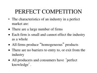
Perfect Competition 1. Buyers and sellers are competitive or price takers 2. All firms produce homogeneous (standardized) goods and consumers view them as identical 3. All buyers and sellers have perfect information regarding the price and quality of the product 4. Firms can enter and exit the industry freely 5. There are no transaction costs to participate in the market 6. Each firm bears the full cost of its production process 7. There is perfect divisibility of output
Competitive agents Large number of agents What really matters are beliefs
Homogeneous Goods Price and nothing else matters The demand for your product goes to zero if you raise price
Perfect Information Buyers and sellers know everything quality opportunities to buy and sell factors affecting the market in the future
Ease of Entry and Exit New firms enter when there are profits Existing firms leave when there are losses
No Transactions Costs Firms are not dissuaded by participation fees Buyers can take advantage of opportunities
No Externalities What is good for this market is good for society The market fully accounts for all costs
Divisible output Small price changes don’t lead to large quantity jumps Examples such as buildings and machinery
Demand facing the perfectly competitive firm The demand curve facing a perfectly competitive firm is horizontal at the market price If the firm were to raise its price, even a tiny bit, above this price, its sales would go to zero And no matter how much the firm produces, this price will not change
Demand for Individual Firm $ p0 D(p) Output Industry Supply-Demand Equilibrium $ S(p) p0 D(p) Output Q0 The demand curve for a perfectly competitive firm is horizontal If the firm were to raise its price above this price, sales would go to zero And no matter how much the firm produces, the price will not change
Behavior of a Single Competitive Firm The firm’s goal is to maximize profit
What is profit? Profit is revenue minus costs or
The firm’s goal is then to maximize returns from the technologies it controls, taking into account: The demandfor final consumption goods Opportunities for buying and selling factors / products The actions of other firms in the market
Example Problem P = $184
yFCVCCAFCAVCATCMC Price TRMRProfit 0.00 2000.00 200.00 1840-200.00 64.00 184.00 1.00 20064.00 264.00 200.00 64.00 264.00 184184-80.00 66.00 184.00 2.00 200130.00 330.00 100.00 65.00 165.00 18436838.00 74.00 184.00 3.00 200204.00 404.00 66.67 68.00 134.67 184552148.00 88.00 184.00 4.00 200292.00 492.00 50.00 73.00 123.00 184736244.00 108.00 184.00 5.00 200400.00 600.00 40.00 80.00 120.00 184920320.00 134.00 184.00 6.00 200534.00 734.00 33.33 89.00 122.33 1841104370.00 166.00 184.00 7.00 200700.00 900.00 28.57 100.00 128.57 1841288388.00 204.00 184.00 8.00 200904.00 1104.00 25.00 113.00 138.00 1841472368.00 248.00 184.00 9.00 2001152.00 1352.00 22.22 128.00 150.22 1841656304.00 298.00 184.00 10.00 2001450.00 1650.00 20.00 145.00 165.00 1841840190.00
TR C Total Revenue and Cost Curves 4000 $ 3500 3000 2500 2000 1500 1000 500 0 0 2 4 6 8 10 12 14 16 18 Output Note that TR is linear with slope = 184
ATC MC Price Price, Marginal Cost, and Average Cost Price = MR = Demand 400 $ 350 300 250 200 150 100 50 0 0 2 4 6 8 10 12 14 16 18 Output
AFC AVC ATC MC Price Add average variable and average fixed costs 400 $ 350 300 250 200 150 100 50 0 0 2 4 6 8 10 12 14 16 18 Output
Maximizing profit Choose the level of output where the difference between TR and TC is the greatest
yCMCPriceTRMRProfit 3 404 184552148 88.00 184.00 4492 184736244 108.00 184.00 5 600 184920320 134.00 184.00 6 734 1841104370 166.00 184.00 7 900 1841288388 204.00 184.00 8 1104 1841472368 248.00 184.00 9 1352 1841656304
Profit Max Using MR and MC An increase in output will always increase profit if MR > MC An increase in output will always decrease profit if MR < MC
The rule is then Increase output whenever MR > MC Decrease output if MR < MC
yCMCPriceTRMRProfit 4.00 492.00 184736244.00 108.00 184.00 5.00 600.00 184920320.00 134.00 184.00 6.00 734.00 1841104370.00 166.00 184.00 7.00 900.00 1841288388.00 204.00 184.00 8.00 1104.00 1841472368.00 248.00 184.00 9.00 1352.00 1841656304.00 Yes Should we increase output from 5 to 6? Yes Should we increase output from 6 to 7? No ! Should we increase output from 7 to 8?
Measuring Total Profit Profit is always given by Graphically it is the distance between total revenue and total cost
TR C Total Revenue and Cost Curves 4000 $ 3500 3000 2500 2000 1500 1000 500 0 0 2 4 6 8 10 12 14 16 18 Output
Profit, price, and average total cost Profit per unit is given by
Cost Curves and Profit ATC MC Price ATC Opt Q Opt $ 350 300 250 200 150 100 50 0 0 2 4 6 8 10 12 14 16 18 Output The distance between price and ATC at the optimum output level is profit per unit
Total profit is given by the area of the box bounded by price, the optimum quantity, average total cost at the optimum quantity, and the price axis
ATC MC Price ATC Opt Q Opt Cost Curves and Profit $ 350 300 250 200 150 100 50 0 0 2 4 6 8 10 12 14 16 18 Output
yCAVCATCMCPriceTRProfit 5.00 600.00 80.00 120.00 184920320.00 134.00 6.00 734.00 89.00 122.33 1841104370.00 166.00 7.00 900.00 100.00 128.571841288388.00 204.00 8.00 1104.00 113.00 138.00 1841472368.00 (184 - 128.5714) = 55.4286 (55.4286) (7) = $388 The firm earns a profit whenever p > ATC
A firm suffers a loss whenever p < ATC at the optimum level of output Let p = $97 We can show that the optimum quantity is 4 units
yCAVCATCMCPriceTRProfit 0.00 200.00 970-200.00 64.00 1.00 264.00 64.00 264.00 9797-167.00 66.00 2.00 330.00 65.00 165.00 97194-136.00 74.00 3.00 404.00 68.00 134.67 97291-113.00 88.00 4.00 492.00 73.00 123.00 97388-104.00 108.00 5.00 600.00 80.00 120.00 97485-115.00 134.00 6.00 734.00 89.00 122.33 97582-152.00 166.00 7.00 900.00 100.00 128.57 97679-221.00
ATC MC Price ATC Opt Loss Q Opt Cost Curves and Profit 400 $ 350 300 250 200 150 100 50 0 0 2 4 6 8 10 12 14 16 18 Output
yFCVCCAFCAVCATCMCPriceTRMRProfit 0.00 2000.00 200.00 970-200.00 64.00 97.00 1.00 20064.00 264.00 200.00 64.00 264.00 9797-167.00 66.00 97.00 2.00 200130.00 330.00 100.00 65.00 165.00 97194-136.00 74.00 97.00 3.00 200204.00 404.00 66.67 68.00 134.67 97291-113.00 88.00 97.00 4.00 200292.00 492.00 50.00 73.00 123.00 97388-104.00 108.00 97.00 5.00 200400.00 600.00 40.00 80.00 120.00 97485-115.00 134.00 97.00 6.00 200534.00 734.00 33.33 89.00 122.33 97582-152.00 166.00 97.00 7.00 200700.00 900.00 28.57 100.00 128.57 97679-221.00 204.00 97.00 8.00 200904.00 1104.00 25.00 113.00 138.00 97776-328.00 248.00 97.00 9.00 2001152.00 1352.00 22.22 128.00 150.22 97873-479.00 298.00 97.00 10.00 2001450.00 1650.00 20.00 145.00 165.00 97970-680.00
Another example problem P = $120
yPriceTRMRFCVCCAFCAVCATCMCProfit 0.00 12001202000.00 200.00 -200.00 0.25 1203012020024.14 224.14 800.00 96.56 896.56 93.19 -194.14 0.50 1206012020046.63 246.63 400.00 93.25 493.25 86.75 -186.63 1.00 12012012020087.00 287.00 200.00 87.00 287.00 75.00 -167.00 2.00 120240120200152.00 352.00 100.00 76.00 176.00 56.00 -112.00 3.00 120360120200201.00 401.00 66.67 67.00 133.67 43.00 -41.00 4.00 120480120200240.00 440.00 50.00 60.00 110.00 36.00 40.00 5.00 120600120200275.00 475.00 40.00 55.00 95.00 35.00 125.00 6.00 120720120200312.00 512.00 33.33 52.00 85.33 40.00 208.00 7.00 120840120200357.00 557.00 28.57 51.00 79.57 51.00 283.00 8.00 120960120200416.00 616.00 25.00 52.00 77.00 68.00 344.00 9.00 1201080120200495.00 695.00 22.22 55.00 77.22 91.00 385.00 10.00 1201200120200600.00 800.00 20.00 60.00 80.00 120.00 400.00 11.00 1201320120200737.00 937.00 18.18 67.00 85.18 155.00 383.00 12.00 1201440120200912.00 1112.00 16.67 76.00 92.67 196.00 328.00 14.00 12016801202001400.00 1600.00 14.29 100.00 114.29 296.00 80.00 16.00 12019201202002112.00 2312.00 12.50 132.00 144.50 420.00 -392.00
For a given price we can find optimal output HOW? Choose output level where MC = MR = P
AVC ATC MC Q Opt P = 120 Profit = $400 Short Run Equilibrium 300 $ 250 200 150 100 50 0 0 2 4 6 8 10 12 14 16 18 Output P = MC y* = 10
yPriceTRMRCostMCProfit 7.00 120840120557.00 51.00 283.00 8.00 120960120616.00 68.00 344.00 9.00 1201080120695.00 91.00 385.00 10.00 1201200120800.00 120.00 400.00 11.00 1201320120937.00 155.00 383.00 12.00 12014401201112.00196.00 328.00 = $400 The firm is happy!! And R - VC (ROVC) = $600
AVC ATC MC Q Opt P = 120 ROVC ROVC = $600 Short Run Equilibrium 300 $ 250 200 150 100 50 0 0 2 4 6 8 10 12 14 16 18 Output P = MC y* = 10
Now let p = $91 y Price TR MR VC C MC Profit 6 91 546 91 312 512 40 34 7 91 637 91 357 557 51 80 8 91 728 91 416 616 68 112 9 91 819 91 495 695 91 124 10 91 910 91 600 800 120 110 11 91 1001 91 737 937 155 64 12 91 1092 91 912 1112 196 -20 y* = 9, = $124 The firm is still happy!! And R - VC (ROVC) = $324