Comparing Means
Comparing Means. Anova. F-test can be used to determine whether the expected responses at the t levels of an experimental factor differ from each other When the null hypothesis is rejected, it may be desirable to find which mean(s) is (are) different, and at what ranking order.

Comparing Means
E N D
Presentation Transcript
Anova • F-test can be used to determine whether the expected responses at the t levels of an experimental factor differ from each other • When the null hypothesis is rejected, it may be desirable to find which mean(s) is (are) different, and at what ranking order. • In practice, it is actually not primary interest to test the null hypothesis, instead the investigators want to make specific comparisons of the means and to estimate pooled error
Means comparison • Three categories: 1. Pair-wise comparisons (Post-Hoc Comparison) 2. Comparison specified prior to performing the experiment (Planned comparison) 3. Comparison specified after observing the outcome of the experiment • Statistical inference procedures of pair-wise comparisons: • Fisher’s least significant difference (LSD) method • Duncan’s Multiple Range Test (DMRT) • Student Newman Keul Test (SNK) • Tukey’s HSD (“Honestly Significantly Different”) Procedure
Pair Comparison Suppose there are t means • An F-test has revealed that there are significant differences amongst the t means • Performing an analysis to determine precisely where the differences exist.
Pair Comparison • Two means are considered different if the difference between the corresponding sample means is larger than a critical number. Then, the larger sample mean is believed to be associated with a larger population mean. • Conditions common to all the methods: • The ANOVA model is the one way analysis of variance • The conditions required to perform the ANOVA are satisfied. • The experiment is fixed-effect.
Comparing Pair-comparison methods • With the exception of the F-LSD test, there is no good theoretical argument that favors one pair-comparison method over the others. Professional statisticians often disagree on which method is appropriate. • In terms of Power and the probability of making a Type I error, the tests discussed can be ordered as follows: MORE PowerHIGHER P[Type I Error] Tukey HSD Test Student-Newman-Keuls Test Duncan Multiple Range TestFisher LSD Test • Pairwise comparisons are traditionally considered as “post hoc” and not “a priori”, if one needs to categorize all comparisons into one of the two groups
Fisher Least Significant Different (LSD) Method • This method builds on the equal variances t-test of the difference between two means. • The test statistic is improved by using MSE rather than sp2. • It is concluded that mi and mj differ (at a% significance level if |mi - mj| > LSD, where
Example: protein source ANOVA Table of CRD Source of Sum of Degrees of Mean Variation Squares Freedom Squares Fcalc. Treatments 216 2 108 18.00 Error 36 6 6 Total 252 8
Duncan’s Multiple Range Test • The Duncan Multiple Range test uses different Significant Difference values for means next to each other along the real number line, and those with 1, 2, … , a means in between the two means being compared. • The Significant Difference or the range value: where ra,p,n is the Duncan’s Significant Range Value with parameters p(= range-value) and n (= MSE degree-of-freedom), and experiment-wise alpha level a (= ajoint).
Duncan’s Multiple Range Test • MSE is the mean square error from the ANOVA table and n is the number of observations used to calculate the means being compared. • The range-value is: • 2 if the two means being compared are adjacent • 3 if one mean separates the two means being compared • 4 if two means separate the two means being compared • …
Student-Newman-Keuls Test • Similar to the Duncan Multiple Range test, the Student-Newman-Keuls Test uses different Significant Difference values for means next to each other, and those with 1, 2, … , a means in between the two means being compared. • The Significant Difference or the range value for this test is • where qa,a,n is the Studentized Range Statistic with parameters p (= range-value) and n (= MSE degree-of-freedom), and experiment-wise alpha level a (= ajoint).
Student-Newman-Keuls Test • MSE is the mean square error from the ANOVA table and n is the number of observations used to calculate the means being compared. • The range-value is: • 2 if the two means being compared are adjacent • 3 if one mean separates the two means being compared • 4 if two means separate the two means being compared • …
Tukey HSD Procedure The test procedure: • Assumes equal number of observation per populations. • Find a critical number w as follows: dft = treatment degrees of freedom n =degrees of freedom = dfe ng = number of observations per population a = significance level qa(dft,n) = a critical value obtained from the studentized range table
Scheffe There are many multiple (post hoc) comparison procedures Considerable controversy: “I have not included the multiple comparison methods of D.B. Duncan because I have been unable to understand their justification”
Planned Comparisons or Contrasts • In some cases, an experimenter may know ahead of time that it is of interest to compare two different means, or groups of means. • An effective way to do this is to use contrasts or planned comparisons. These represent specific hypotheses in terms of the treatment means such as:
Planned Comparisons or Contrasts • Each contrast can be specified as:and it is required: • A sum-of-squares can be calculated for a contrast as
Planned Comparisons or Contrasts • Each contrast has 1 degree-of-freedom, and a contrast can be tested by comparing it to the MSE for the ANOVA: • If more than 1 contrast is tested, it is important that the contrasts all be orthogonal, that is Note that It can be tested at most t-1 orthogonal contrasts.
Orthogonal Polynomials • Special sets of coefficients that test for bends but manage to remain uncorrelated with one another. • Sometimes orthogonal polynomials can be used to analyze experimental data to test for curves. • Restrictive assumptions: • Require quantitative factors • Equal spacing of factor levels (d) • Equal numbers of observations at each cell (rj) • Usually, only the linear and quadratic contrasts are of interest
Orthogonal Polynomial • The linear regression model y = X + is a general model for fitting any relationship that is linear in the unknown parameter . • Polynomial regression model:
Polynomial Models in One Variable • A second-order model (quadratic model):
A second-order model (quadratic model)
Polynomial Models • Polynomial models are useful in situations where the analyst knows that curvilinear effects are present in the true response function. • Polynomial models are also useful as approximating functions to unknown and possible very complex nonlinear relationship. • Polynomial model is the Taylor series expansion of the unknown function.
Choosing order of the model • Theoretical background • Scatter diagram • Orthogonal polynomial test