Download
1 / 34
340 likes | 395 Vues
Explore the impact of solar irradiance changes on climate, from measurements to reconstructions and simulations with climate models. Discover the historical significance and modern implications of solar activity on Earth's climate system.

E N D
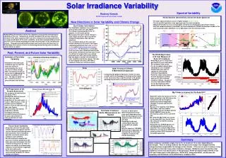
Solar Irradiance Variability and Climate Claus Fröhlich Physikalisch-Meteorologisches Observatorium Davos World Radiation Center CH 7260 Davos Dorf With contributions from Joanna Haigh, Judith Lean, Mike Lockwood and Simon Foster, Eugene Rozanov and Tania Egorova 35thCOSPAR 2004, Paris, Interdisciplinary Lecture, 23 July 2004
Outline • Introduction • Solar Irradiance Changes: Measurements • Total solar irradiance • Spectral solar irradiance • Solar Irradiance Changes: Mechanisms and Models • Sunspot and faculae • Network inside and outside active regions • Relation to solar surface magnetic fields • Solar Irradiance Changes:Reconstructions for the past • Proxies for solar activity: sunspot numbers, cosmogenic isotopes • What can we learn from solar-like stars? • Solar irradiance re-constructions • Climate change due to solar irradiance variability • Simulations with climate models • Comparisons with Observations • Conclusions 35thCOSPAR 2004, Paris, Interdisciplinary Lecture, 23 July 2004
Introduction (1 of 4) • Total solar irradiance (TSI) is the main power for the Earth-atmosphere system. Hence even small changes of TSI have the potential to change our climate. • 0.1% change of the solar constant yields a climate forcing of 1.365x0.7/4 = 0.24 Wm-2. This amount of forcing equals the forcing of recent 5-year increase of greenhouse gases – so it is small! • Due to the large inertia of the oceans changes on up to decadal scales – as e.g the solar cycle variation – are strongly attenuated, whereas changes on longer time-scales may well contribute global change if they exist. 35thCOSPAR 2004, Paris, Interdisciplinary Lecture, 23 July 2004
Introduction (2 of 4) • Although the ‚Solar Constant Program‘ of the Smithsonian Astrophysical Observatory was founded for the detection of solar irradiance changes and operated for more than half a century, only modern satellite measurements were able to uniquely identify changes of TSI. • A possible connection between solar activity and climate and/or weather was speculated since the 11-year cycle of solar activity was detected by Schwabe. ,,,,,,,,,,with many failures, however. • The detection of TSI being higher during high activity brought new ideas about solar-climate connection mainly due to the coincidence of the ‚Little Ice Age‘ and the Maunder Minimum of solar activityin the 17th century (e.g. Eddy, 1976) 35thCOSPAR 2004, Paris, Interdisciplinary Lecture, 23 July 2004
Introduction (3 of 4) • The 11-year solar cycle as represented by the sunspot number varies strongly. A indicates the Maunder, B the Dalton Minimum and C the present maximum • The solar activity record of sunspot numbers can be extended by the cosmogenic isotopes. • Also the Earth‘ climate changes. Represented here as anomaly of the NH surface temperature 35thCOSPAR 2004, Paris, Interdisciplinary Lecture, 23 July 2004
Introduction (4 of 4) A major question is, how much of the climate change during the lastmillennium is due to the Sun and how much is anthropogenic. As the positive and negative forcings are almost balancedthe Sun may still play arole from the mid of the 18th to the mid of the 20th century although the forcing is rather small. 35thCOSPAR 2004, Paris, Interdisciplinary Lecture, 23 July 2004
Observations of Solar Influence for the Present • Signatures of solar influence are searched with a multi-factorial analysis of data from the last few solar activity cycles • For the stratosphere F10.7, QBO, a linear trend, and volcanic effects are included • Stratospheric temperature from rocket data 1969-1990s • Ozone mixing ratio from SAGE II • For the troposphere the following effects have to be added: El Nino, NAO and 4 indices for annual and semi-annual periodicities • Temperature from NCEP re-analysis 1979-2000 • Mean zonal wind from NCEP re-analysis 1979-2002 35thCOSPAR 2004, Paris, Interdisciplinary Lecture, 23 July 2004
TSI Database 1978 to present: What is available and which data contribute to the composite? • Since 1978 reliable TSI measurements from space are available from the following overlapping missions with electrically calibrated radiometers (ECR): • HF (Hickey-Frieden) on NIMBUS7 (17/11/1978 - 24/01/1993) • ACRIM-I on SMM (16/02/1980 - 01/06/1989) • ERBE on ERBS (24/10/1984 - 12/03/2003) • ACRIM-II on UARS (06/10/1991 - 27/09/2001) • SOVA on EURECA (11/08/1992 - 15/05/1993) • VIRGO on SOHO (07/02/1996 - ………) • ACRIM-III on AcrimSat (05/04/2000 – ………) • TIM on SORCE (25/02/2003 - ………) • For the composite results from HF, ACRIM-I and II and VIRGO are used, with ACRIM-I as radiometric reference. • ERBE data are used as an independent dataset for comparison. As its sampling is so sparse (once every 14 days for a few minutes) daily data from a proxy model are also used for interpolation between the measured ERBE points. 35thCOSPAR 2004, Paris, Interdisciplinary Lecture, 23 July 2004
TSI Database 1978 to present: What can be learned from VIRGO • The performance of radiometers in space can be illustrated with the results from the VIRGO experiment on SOHO: • Level 1 data show quite different long-term behavior. Note the early increase of PMO6V radiometers. • Corrections for exposure- dependent changes are determined by comparison with less exposed radiometers. These changes can be described for PMO6V with hyperbolic functions of the exposure dose. The behavior of DIARAD is not well understood. • By comparison of the time series of the two radiometer types for exposure dependent effects some exposure independent changes can be identified for DIARAD, but not for PMO6V. The latter is an important result because PMO6V is similar to ACRIM, HF and ERBE as far as the paint in the cavity is concerned. 35thCOSPAR 2004, Paris, Interdisciplinary Lecture, 23 July 2004
TSI Database 1978 to present: Corrections needed for the Composite • All data sets need some corrections which will be explained shortly: • VIRGO data are correctedfor degradation • ACRIM-I data need a change in the timely distribution of the early degradation • HF data need to be corrected for degradation, some glitches and a trend which is not exposure dependent • ACRIM-II have some glitches and the level has to be adjusted to the level of ACRIM-I • The HF and VIRGO data have to be shifted to the level of ACRIM-Iwhich is the radiometric referencefor the PMOD composite 35thCOSPAR 2004, Paris, Interdisciplinary Lecture, 23 July 2004
TSI Database 1978 to present: Discussion of the PMOD and ACRIM composites A major result of the PMOD composite is that the Sun did not change during the last 25 years. If the HF correction during the gap between ACRIM I and II is neglected, one gets the ACRIM composite. Comparison of both composites with ERBS shows convincing evidence for the need of the HF correction and disproves the statement that ERBS was degrading. Moreover, the steady increase of the ratio is compatible with the early increase of the PMO6V radiometers: With a total of 2.6 days of exposure the observed early trend becomes 210 ppm per exposure day which compares very well with 184 ppm for PMO6V-A observed at the beginning of its exposure on SOHO. Comparison with a proxy model supports this conclusion – but they are not used as argument! The composite and VIRGO data are available from www.pmodwrc.ch 35thCOSPAR 2004, Paris, Interdisciplinary Lecture, 23 July 2004
Estimation of the Uncertainty of the Composite TSI and of a Possible Trend • In order to asses the long-term uncertainty of the composite we may use the uncertainty of the slope of the comparison with ERBE which amounts to 4 ppm/a or 42 ppm over the time between the minima. Although this uncertainty is mainly due to the sampling noise in the ERBE data (Spearman rank =0.773) it may be used as an upper limit. The difference in slope of the two composite is mainly due to the corrections of ACRIM-II not considered in the ACRIM composite. • The uncertainty of the HF corrections over the ACRIM gap amounts to 51 ppm. • The trend determined by the difference of the two minima is –33ppm with a formal error of 5 ppm. Together with the uncertainty of the corrections over the ACRIM gap (51 ppm), the trend is not significance at the 2 level, and if the uncertainty from ERBE comparison is included at the 2.2 level. • This uncertainty is astoundingly low compared to the estimated absolute uncertainty at the 1500 ppm level and only possible because we had during the whole period always overlapping measurements from two or more simultaneous missions. • Results from TIM on SORCE are lower by about 0.3%. It may indicate that the absolute uncertainty of the present radiometers used in space is underestimated or some effects not accounted for. 35thCOSPAR 2004, Paris, Interdisciplinary Lecture, 23 July 2004
Spectral Distribution of Solar Irradiance The reason for the Sun not being a black body radiator is the spectrally varying opacity of the solar atmosphere. The opacity determines the formation height of the radiation and thus its emission from the temperture of the solar atmosphere. 35thCOSPAR 2004, Paris, Interdisciplinary Lecture, 23 July 2004
Spectral Irradiance Variability (1 of 2) • At present the longest and most reliable data are the measure-ments made by SOLSTICE and SUSIM on UARS, since October 1991. Prior to UARS, SME monitored the UV irradiance with lesser accuracy and precision. The UARS and SME data suggest solar cycle irradiance changes of 20%, 8% and 3% near 140, 200 and 250 nm, respectively. • The spectral irradiance variability during the 11-year solar cycle in terms of percentage changes and also as energy changes show the strong wavelength dependence of the variations. Rotational modulation of spectral irradiance is super-imposed on the solar cycle variations at all wavelengths. 35thCOSPAR 2004, Paris, Interdisciplinary Lecture, 23 July 2004
Spectral Irradiance Variability (2 of 2) • VIRGO on SoHO monitors spectral irradiance with filterradiometers (SPM) at 402, 500 and 862 nm with 5nm bandwidth. • Although the long-term degradation cannot be accounted for completely the time series are represen-tative for periods shorter than about 400 days. • The TSI time series is detrended the same way for comparison. 35thCOSPAR 2004, Paris, Interdisciplinary Lecture, 23 July 2004
Power Spectra of Irradiance Variability • The power spectrum of TSI includes periods up to the solar cycle from the composite and down to the 5-minute oscillations from the VIRGO data. The latter time series allows also comparison of a quiet and active Sun. • The power spectra of the VIRGO/SPM show how variable it is as a function of wavelength. • An interesting result is the ratio of active to quiet solar irradiance power. • From these power spectra the spectral redistribution of power can also be determined. 35thCOSPAR 2004, Paris, Interdisciplinary Lecture, 23 July 2004
Origin of Irradiance Variability • Solar activity, initially detected in sunspot observations in the mid nineteenth century originates in a cycle of magnetic flux driven by a dynamo seated near the bottom of the convection zone. • This flux produces a variety of features, such as sunspots, faculae and plages, and instigates numerous solar phenomena, including irradiance and solar wind fluctuations, flares and coronal mass ejections. • There may be other effects such as temperature, radius and other changes in the interior of the Sun which may alter the irradiance. • Although the solar magnetic cycle is most probablythe ultimate driver of irradiance variations, solar irradiance correlates poorly with the net and disk-averaged magnetic flux. Only 18 and 3% of the TSI variance are explained. 35thCOSPAR 2004, Paris, Interdisciplinary Lecture, 23 July 2004
Influence of Sunspots and Faculae • The series of images (July 1988) illustrates the darkening of sunspots and brightening by faculae • The two different effects modulating the irradiance are obvious also from the histograms of the variance. The ratio of the two effects varies within the cycle. • From the position of the maximum of the distribution the relative contributions of sunspots and faculae can be determined. 35thCOSPAR 2004, Paris, Interdisciplinary Lecture, 23 July 2004
Proxy Model of Irradiance Variations (1 of 5) • Sunspots can be modeled from their area and position on the disk by using an appropriate contrast. The result is the photometric sunspot index (PSI) • For faculae a similar approach could be applied. However, the areas are difficult to observe directly. So they have to derived from plages, magnetograms or spot areas. Here, we use the Mg Index as a surrogate for faculae and network • The Mg index can easily be devided into short and long-term parts representing the faculae and network within and outside active regions. 35thCOSPAR 2004, Paris, Interdisciplinary Lecture, 23 July 2004
Proxy Model of Irradiance Variations (2 of 5) • The model is calibrated by regression of the three components PSI, MgIIst and MgIIlt with the TSI composite. The resulting parameters are -1.03 ±0.01, 80.3±1.3, 120.3 ±0.9, respectively. The result can be improved by calibrating each cycle separately with changes of the parameters by up to 10% for PSI and MgIIst The model explains 78% of the variance. • Comparison with the mode results shows interesting differences which may be important for future improvement of the model. 35thCOSPAR 2004, Paris, Interdisciplinary Lecture, 23 July 2004
Proxy Model of Irradiance Variations (3 of 5) • Another way to judge the correlation is from the results of bi-variate spectral analysis. • On average the correlation of 0.833 is confirmed. However, much lower correlations are found at various periods, among others around 500 days and at the 27-day solar rotation period. 35thCOSPAR 2004, Paris, Interdisciplinary Lecture, 23 July 2004
Proxy Model of Irradiance Variations (4 of 5) • A similar model can be developed for spectral irradiance. • The contrasts for sunspots and faculae are from theoretical calculations • The results are from a 2-component model with PSI and a facular index from Ca images calibrated against the corresponding UARS-SOLSTICE time series. 35thCOSPAR 2004, Paris, Interdisciplinary Lecture, 23 July 2004
Proxy Model of Irradiance Variations (5 of 5) • A 3-component model for TSI with PSI, short and long-term Mg index can explain 78% of the variance. A 2-component model with PSI and the Mg index yields a somewhat smaller correlation. • The 2-component model for the spectral irradiance is less accurate, mainly because of the larger uncertainty of the spectral measurements and also because of the uncertainty of the contrasts. • The sunspot component is well understood and PSI is quite reliable. Improvements could be incorporated by including a solar cycle dependent contrast, as suggested by photometric observations and the comparison with the mode. • It is interesting that the MgII Index works so well although it cannot reproduce several details properly as e.g. the center-to-limb dependence.The correlation can be improved by filtering TSI+PSI and MgIIst by appropriate functions (camel for the former and dromedary for the latter) 35thCOSPAR 2004, Paris, Interdisciplinary Lecture, 23 July 2004
Reconstruction of Irradiance Variations in the Past (1 of 7) • The Zürich sunspot numbers were defined by Wolf and are well representing the strength of the solar cycle and not so much the influence of sunspots • The cosmogenic isotopes vary in a similar way as the solar cycle amplitude of the sunspot number. This suggests that they might be used to infer the level of solar activity over even longer periods.They are produced by galactic cosmic rays which are modulated at Earth by the interplanetary magnetic field • The interplanetary magnetic field is determined by the open flux leaving the Sun and is monitored on Earth by e.g. the AA Index since 1868. 35thCOSPAR 2004, Paris, Interdisciplinary Lecture, 23 July 2004
Reconstruction of Irradiance Variations in the Past (2 of 7) Past irradiance variations are reconstructed according to the following schemes: • Reconstruct the 11-year solar cycle variations. One method is based on the sunspot numbers calibrated in terms of irradiance by fitting the last three cycles to the composite. This provides a record back to the late 16th century. Another method is using a model for facular brightening and the sunspot areas and locations of the Greenwich observations back to the late 19th century. • Add a secular change (background) which follows e.g. the sunspot number envelope amplitude or the solar cycle length. The magnitude of the change between the Maunder Minimum and today is a free parameter and is determined by comparison with stellar analogues or from the irradiance of a magnetically free Sun. • Note that all the reconstructions are implicitly assuming that the Sun has the same features as observed during the last 25 years 35thCOSPAR 2004, Paris, Interdisciplinary Lecture, 23 July 2004
Reconstruction of Irradiance Variations in the Past (3 of 7) • From MDI magnetograms one can determine the distribution of the radial magnetic field within an active region. From such distributions the facular pixels are selected according to 60G<B/<200G. Inside and outside active regions pixel with B/<60G are classified as network. Summing up the selected pixels and applying a corresponding -dependent contrast determined from the MDI continuum images (Ortiz et al. 2000) the facular and network contributions within an active region can be estimated • For averages over periods longer than the 27-day rotation the facular area is linearly correlated with the observed sunspot area (r=0.92) of the active region. Based on this correlation and with the -dependent contrast the facular brightening can be calculated. • Summing up the quiet sun pixels outside the active region and using the network contrast the solar minimum value can be determined and extrapolated to zero magnetic field. 35thCOSPAR 2004, Paris, Interdisciplinary Lecture, 23 July 2004
Reconstruction of Irradiance Variations in the Past (4 of 7) Now we compare the results from the solar cycle (short term) reconstructions by Lean 2000 and Foster 2004 35thCOSPAR 2004, Paris, Interdisciplinary Lecture, 23 July 2004
Q0 Reconstruction of Irradiance Variations in the Past (5 of 7) What can we learn from solar-type stars for possible secular trends (background)? • Originally the picture from the Mount-Wilson Program showed convincing evidence of a Maunder-Minimum state of the Sun. • More recent data from the open cluster M67 and a detailed re-analysis of the Mount-Wilson data in terms of solar analogues does no longer support the bimodal distribution • The Q0 value of a magnetically free Sun coincides approximately with the minimum value of the solar twins of M67.. 35thCOSPAR 2004, Paris, Interdisciplinary Lecture, 23 July 2004
Reconstruction of Irradiance Variations in the Past (6 of 7) • The reconstruction of Foster 2004 is based on the fact that the Sun still had some magnetism during the Maunder Minimum as manifested by the 10Be record. So, he lets the background contribution to go half way down to Q0. • Comparison of the Foster reconstruction (blue) with trend Q0/2, with no trend (mauve) and with full trend to Q0.. The blue line is from the aa-index fitted to the composite. 35thCOSPAR 2004, Paris, Interdisciplinary Lecture, 23 July 2004
Reconstruction of Irradiance Variations in the Past (7 of 7) In a similar way the spectral irradiance can be reconstructed. However, the work of Foster 2004 suggests to scale the values according to represent the background change from present to the Maunder Minimum as Q0/2. So the quoted percent values have to be devided by 2 35thCOSPAR 2004, Paris, Interdisciplinary Lecture, 23 July 2004
Comparison with Climate Models (1 of 3) Comparison of model simulationsfor the H&S and LBB reconstructions of the late nineties with ECHAM3 (from Cubasch et al 2000) and with the GISS model (from Shindell et al. 2001) 35thCOSPAR 2004, Paris, Interdisciplinary Lecture, 23 July 2004
Comparison with Climate Models (2 of 3) Recent simulations with the GISS GCMAM which includes spectral changes from Lean 2000 and calculates Ozone yield the following results for the Maunder Minimum period (from Rind et al., 2004): • Spectrally differentiated irradiance compared with percentage change of TSI does not change the response of the surface temperature drastically. • The reduced UV radiation reduces Ozone, but the pre-industrial atmospheric composition increases it slightly • The calculated cooling is much stronger than estimated from temperature reconstructions 35thCOSPAR 2004, Paris, Interdisciplinary Lecture, 23 July 2004
Comparison of Model Simulations with Observations An interesting example of the influence of spectrally differentiated irradiance changes from min to max of the solar cycle are from simulations with SOCOL which couples MAECHAM4 with a chemistry transport model MEZON (from Egorova et al., 2003) • Influence of max-to-min change of the spectral irradiance in the UV and visible on the NH surface temperature • Stratospheric temperature change between max and min in red; in blue the control run and green the result after 1 year. • Comparison with SSU/MSU (blue), CPC re-analysis (cyan), NCEP re-analysis (green), MAECHAM/CHEM simulations (magenta) show that there are is still room for improvements 35thCOSPAR 2004, Paris, Interdisciplinary Lecture, 23 July 2004
Conclusions • Solar irradiance changes with the 11-year solar cycle, being higher during solar maximum (ca. 0.1% for TSI) • During the last 25 years of space measurements no trend can be inferred from the composite time series • The last 25 years of TSI and also SSI can be satisfactorily modeled with 2-3 component proxy models describing the sunspot darkening and the brightening by faculae and network. • Reconstructions are built with the understanding of the present Sun and the behavior during the last 3 activity cycles – but with more weight on cycle 23 which is regarded as rather unusual. The present understanding postulates a TSI during the Maunder Minimum which is only about 0.8 Wm-2 lower than during present minima. Earlier reconstruction assumed much larger dimming. • Simulations with climate models using 2.5-5.0 Wm-2 TSI change overestimate the reconstructed temperature change. Including spectral changes does improve the results in several aspects, but the understanding of the details of how irradiance variability changes climate is far from being perfect. 35thCOSPAR 2004, Paris, Interdisciplinary Lecture, 23 July 2004