Digital Communications Tutorial
Digital Communications Tutorial. Cognitive Radio Communications @ Virginia Tech NSF Research Experiences for Undergraduates (REU) Site Ratchaneekorn (Kay) Thamvichai tkay@vt.edu. Outline. Introduction Fourier Transform Sampling Pulse Amplitude Modulation (PAM)

Digital Communications Tutorial
E N D
Presentation Transcript
Digital Communications Tutorial Cognitive Radio Communications @ Virginia Tech NSF Research Experiences for Undergraduates (REU) Site Ratchaneekorn (Kay) Thamvichai tkay@vt.edu
Outline • Introduction • Fourier Transform • Sampling • Pulse Amplitude Modulation (PAM) • InterSymbol Interference (ISI) • Digital Bandpass Modulation
Analog vs. Digital • Transmitted bits can be detected and regenerated, so noise does not propagate additively. • More signal processing techniques are available to improve system performance: source coding, channel (error-correction) coding, equalization, encryption, filtering,… • Digital ICs are inexpensive to manufacture • Digital communications permits integration of voice, video, and data on a single system (ISDN) • Implementation of various algorithms can be done by software instead of hardware • Security is easier to implement.
Fourier Transform • F() is the continuous-time Fourier transform of f(t). • The Fourier transformation F(ω) is the frequency domain representation of the original function f(t). It describes which frequencies are present in the original function.
Example 1: x(t) t=0 Ex A: Find the Fourier Transform of x(t) = (t) Ex B: Find the Fourier Transform of x(t) = 0.5cos(500pt)
sinc(x) 1 x -3p -2p -p 0 p 2p 3p sinc function sinc(x) = sin(x) x • even function • zero crossings at • Amplitude decreases proportionally to 1/x
Ex D: Pulsed Cosine: cos(w0t)rec(t/T) <=> (T/2) sinc(w-w0)T + sinc(w+w0)T 2 2
Linear Time-Invariant (LTI) system h(t) Convolution: y(t) = x(t)*h(t) Its Fourier Transform: Y(ω) = X(ω)H(ω) where H(ω) is a frequency response or a transfer function of a system h(t).
Ideal filters • A filter is used to eliminate unwanted parts of the frequency spectrum of a signal. • A filter is LTI system with an impulse response h(t). • The output y(t) of a filter can be founded in time domain using a convolution. • However, it is easier to do it in a frequency domain: Y(ω) = X(ω)H(ω)
Low Pass Filterwith a cutoff frequency wc High Pass Filter
Example 2: Given x(t) = cos(500pt)cos(1000pt), find an impulse response h(t) of a low-pass filter that passes the low frequency component of the signal. x(t) y(t) = low freq. component of x(t) Low-pass filter h(t)
H(w) Y(w) = H(w)X3(w) = p/2[d(w-500p) + d(w+500p)] => y(t) = 0.5cos(500pt) H(w ) = rect(w/2000p) => h(t) = 1000sinc(1000t)
Outline • Introduction • Fourier Transform • Sampling • Pulse Amplitude Modulation (PAM) • InterSymbol Interference (ISI) • Digital Bandpass Modulation
Sampling Continuous-Time signals Sampling – generating of an ordered number of sequence by taking values of f(t) as specified instants of time i.e. f(t1), f(t2), f(t3), … where tm are instants at which sampling occurs. Sampling operation is implemented in hardware by an analog-to-digital converter (ADC) – electronic device used to sample physical voltage signals. In most cases, continuous-time signals are sampled at equal increments of time. The sample increment, called sample period, is usually denoted as Ts.
Impulse sampling Define the continuous time impulse train as: p(t) is an infinite train of continuous time impulse functions, spaced Ts seconds apart.
Let x(t) be a continuous time signal we wish to sample. We will model sampling as multiplying a signal x(t) by p(t).
Sampling Theorem let P(ω) be a Fourier Transform of p(t), X(ω) be a Fourier Transform of x(t), Xs(ω) be a Fourier Transform of xs (t), Since xs(t) = x(t)p(t) by a multiplication property (Fourier Transform),
where Ck are the Fourier Series coefficients of the periodic signal.
We see that an impulse train in time, p(t), has a Fourier Transform that is an impulse train in frequency, P(w). • The spacing between impulses in time is Ts, and the spacing between impulses in frequency is ω0 = 2p/Ts. Note: If we increase the spacing in time between impulses, this will decrease the spacing between impulses in frequency, and vice versa.
Spectrum of a sampled signal replicated scaled versions of X(w), spaced every w0 apart in frequency
Time-domain Frequency-domain ω0 = 2p/Ts
If w0-wc < wc , ALIASING (overlap area) occurs If w0-wc ≥ wc , Note: if ω0 - ωc ≥ ωc orω0 ≥ 2ωc, there is no aliasing
Sampling Theorem Let x(t) be a band-limited signal with X(ω) = 0 for |ω| > ωc. Then x(t) is uniquely determined by its samples x(nTs), n = 0, ±1, ± 2, … if ω0 ≥ 2ωc where ω0 = 2p/Ts. • This is how to choose a sampling frequency (fs = 1/Ts) or period (Ts) such that an original continuous-time signal x(t) can be recovered from a sampled version xs(t). => a sampling rate (ω0) MUST be at least twice the highest frequency (ωc) of a signal to avoid aliasing problem.
To recover x(t) from its sampled version xs(t), we use a low pass filter (reconstruction filter) to recover the center island of Xs(w):
Ex: Given a signal x(t) with Fourier Transform with cutoff frequency ωc as shown: Given three different pulse trains with periods Draw the sampled spectrum in each case. Which case(s) experiences aliasing?
Aliasing Phenomenon • Sampling theorem: the signal is strictly band-limited (wc). However, in practice, no information-bearing signal is strictly band-limited. • Aliasing is the phenomenon of a high-frequency component in the spectrum of the signal seemingly taking on the identify of a lower frequency in the spectrum of its sampled version. • To prevent the effects of aliasing in practice • Prior to sampling : a low-pass anti-alias filter is used to attenuate those high-frequency components of a message signal that are not essential to the information being conveyed by the signal. • The filtered signal is sampled at a rate slightly higher than the Nyquist rate.
Example: Why 44.1 kHz for Audio CDs? • Sound is audible in 20 Hz to 20 kHz range: fmax = 20 kHz and the Nyquist rate 2fmax = 40 kHz • What is the extra 10% of the bandwidth used? Rolloff from passband to stopband in the magnitude response of the anti-aliasing filter. • Okay, 44 kHz makes sense. Why 44.1 kHz? At the time the choice was made, only recorders capable of storing such high rates were VCRs. • NTSC: 60-Hz video (30 frames/s) - 490 lines per frame or 245 lines per field, 3 audio samples per line the sampling rate is 60 X 245 X 3 = 44.1 KHz
Outline • Introduction • Fourier Transform • Sampling • Pulse Amplitude Modulation (PAM) • InterSymbol Interference (ISI) • Digital Bandpass Modulation
Pulse-Amplitude Modulation (PAM) • The amplitude of regularly spaced pulses are varied in proportion to the corresponding sample values of a continuous message signal. • Two operations involved in the generation of the PAM signal • Instantaneous sampling of the message signal m(t) every Ts seconds, • Lengthening the duration of each sample, so that it occupies some finite value T.
Sample-and-Hold Filter : Analysis • The PAM signal is • The h(t) is a standard rectangular pulse of unit amplitude and duration • The instantaneously sampled version of m(t) is
To modify mδ(t) so as to assume the same form as the PAM signal: • The PAM signal s(t) is mathematically equivalent to the convolution of mδ(t) , the instantaneously sampled version of m(t), and the pulse h(t). • Its Fourier Transform:
One benefit of PAM It enables the simultaneous transmission of multiple signals using time-division multiplexing (TDM). User 1 User 2
Quantization Process • Amplitude quantization: The process of transforming the sample amplitude m(nTs) of a baseband signal m(t) at time t=nTs into a discrete amplitude v(nTs) taken from a finite set of possible levels. It will be represented by binary number(s)
Outline • Introduction • Fourier Transform • Sampling • Pulse Amplitude Modulation (PAM) • MATLAB! • InterSymbol Interference (ISI) • Digital Bandpass Modulation
Baseband Transmission of Digital Data • The transmission of digital data over a physical communication channel is limited by two unavoidable factors • Intersymbol interference • Channel noise
The level-encoded signal and the discrete PAM signal are • The transmitted signal is • The channel output is • The output from the receive-filter is
The InterSymbol Interference (ISI) Problem We may express the receive-filter output as the modified PAM signal where After sampling:
ISI (cont.) Define where E is the transmitted signal energy / bit (symbol). What we desire is However, from Residual phenomenon, intersymbol interference (ISI)
Pulse-shaping • Given the channel transfer function, determine the transmit-pulse spectrum and receive-filter transfer function so as to satisfy two basic requirements: • Intersymbol interference (ISI) is reduced to zero. • Transmission bandwidth is conserved.
The Nyquist Channel • The optimum solution for zero ISI at the minimum transmission bandwidth possible in a noise-free environment • For zero ISI, it is necessary for the overall pulse shape p(t) and the inverse Fourier transform of the pulse spectrum P(f) to satisfy the condition
The overall pulse spectrum is defined by the optimum brick-wall function: • The brick-wall spectrum defines B0 as the minimum transmission bandwidth for zero intersymbol interference. • The optimum pulse shape is the impulse response of an ideal low-pass channel with an amplitude response Popt(f) in the passband and a bandwidth B0
Symbol 2 Symbol 1 Symbol 3