Data Pre-processing
Data Pre-processing. Data cleaning Fill in missing values, smooth noisy data, identify or remove outliers, and resolve inconsistencies Data integration Integration of multiple databases, data cubes, or files Data transformation Normalization and aggregation Data reduction


Data Pre-processing
E N D
Presentation Transcript
Data Pre-processing • Data cleaning • Fill in missing values, smooth noisy data, identify or remove outliers, and resolve inconsistencies • Data integration • Integration of multiple databases, data cubes, or files • Data transformation • Normalization and aggregation • Data reduction • Obtains reduced representation in volume but produces the same or similar analytical results • Data discretization • Part of data reduction but with particular importance, especially for numerical data
Why Data Preprocessing? • Data in the real world is dirty • incomplete: lacking attribute values, lacking certain attributes of interest, or containing only aggregate data • noisy: containing errors or outliers • inconsistent: containing discrepancies in codes or names • No quality data, no quality mining results! • Quality decisions must be based on quality data • Data warehouse needs consistent integration of quality data
Data Cleaning • Data cleaning tasks • Fill in missing values • Identify outliers and smooth out noisy data • Correct inconsistent data
Missing Data • Data is not always available • E.g., many tuples have no recorded value for several attributes, such as customer income in sales data • Missing data may be due to • equipment malfunction • inconsistent with other recorded data and thus deleted • data not entered due to misunderstanding • certain data may not be considered important at the time of entry • not register history or changes of the data • Missing data may need to be inferred.
How to Handle Missing Data? • Fill in the missing value manually: tedious + infeasible? • Use a global constant to fill in the missing value: e.g., “unknown”, a new class?! • Use the attribute mean to fill in the missing value • Use the attribute mean for all samples belonging to the same class to fill in the missing value: smarter • Use the most probable value to fill in the missing value: inference-based such as Bayesian formula or decision tree
Noisy Data • Noise: random error or variance in a measured variable • Incorrect attribute values may due to • faulty data collection instruments • data entry problems • data transmission problems • technology limitation • inconsistency in naming convention • Other data problems which requires data cleaning • duplicate records • incomplete data • inconsistent data
How to Handle Noisy Data? • Binning method: • first sort data and partition into (equi-depth) bins • then one can smooth by bin means, smooth by bin median, smooth by bin boundaries, etc. • Clustering • detect and remove outliers • Combined computer and human inspection • detect suspicious values and check by human • Regression • smooth by fitting the data into regression functions
Simple Discretization Methods: Binning • Equal-width (distance) partitioning: • It divides the range into N intervals of equal size: uniform grid • if A and B are the lowest and highest values of the attribute, the width of intervals will be: W = (B-A)/N. • The most straightforward • But outliers may dominate presentation • Skewed data is not handled well. • Equal-depth (frequency) partitioning: • It divides the range into N intervals, each containing approximately same number of samples • Good data scaling • Managing categorical attributes can be tricky.
Binning Methods for Data Smoothing * Sorted data for price (in dollars): 4, 8, 9, 15, 21, 21, 24, 25, 26, 28, 29, 34 * Partition into (equi-depth) bins: - Bin 1: 4, 8, 9, 15 - Bin 2: 21, 21, 24, 25 - Bin 3: 26, 28, 29, 34 * Smoothing by bin means: - Bin 1: 9, 9, 9, 9 - Bin 2: 23, 23, 23, 23 - Bin 3: 29, 29, 29, 29 * Smoothing by bin boundaries: - Bin 1: 4, 4, 4, 15 - Bin 2: 21, 21, 25, 25 - Bin 3: 26, 26, 26, 34
Regression y Y1 y = x + 1 Y1’ x X1
Data Integration • Data integration: • combines data from multiple sources into a coherent store • Schema integration • integrate metadata from different sources • Entity identification problem: identify real world entities from multiple data sources, e.g., A.cust-id B.cust-# • Detecting and resolving data value conflicts • for the same real world entity, attribute values from different sources are different • possible reasons: different representations, different scales, e.g., metric vs. British units
Handling Redundant Data • Redundant data occur often when integration of multiple databases • The same attribute may have different names in different databases • One attribute may be a “derived” attribute in another table, e.g., annual revenue • Redundant data may be able to be detected by correlational analysis • Careful integration of the data from multiple sources may help reduce/avoid redundancies and inconsistencies and improve mining speed and quality
Data Transformation • Smoothing: remove noise from data • Aggregation: summarization, data cube construction • Generalization: concept hierarchy climbing • Normalization: scaled to fall within a small, specified range • min-max normalization • z-score normalization • normalization by decimal scaling • Attribute/feature construction • New attributes constructed from the given ones
Data Transformation: Normalization • min-max normalization • z-score normalization • normalization by decimal scaling Where j is the smallest integer such that Max(| |)<1
Data Reduction Strategies • Warehouse may store terabytes of data: Complex data analysis/mining may take a very long time to run on the complete data set • Data reduction • Obtains a reduced representation of the data set that is much smaller in volume but yet produces the same (or almost the same) analytical results • Data reduction strategies • Data cube aggregation • Dimensionality reduction • Numerosity reduction • Discretization and concept hierarchy generation
Dimensionality Reduction • Feature selection (i.e., attribute subset selection): • Select a minimum set of features such that the probability distribution of different classes given the values for those features is as close as possible to the original distribution given the values of all features • reduce # of patterns in the patterns, easier to understand • Heuristic methods (due to exponential # of choices): • step-wise forward selection • step-wise backward elimination • combining forward selection and backward elimination • decision-tree induction
> Example of Decision Tree Induction Initial attribute set: {A1, A2, A3, A4, A5, A6} A4 ? A6? A1? Class 2 Class 2 Class 1 Class 1 Reduced attribute set: {A1, A4, A6}
Data Compression • String compression • There are extensive theories and well-tuned algorithms • Typically lossless • But only limited manipulation is possible without expansion • Audio/video compression • Typically lossy compression, with progressive refinement • Sometimes small fragments of signal can be reconstructed without reconstructing the whole • Time sequence is not audio • Typically short and vary slowly with time
Data Compression Original Data Compressed Data lossless Original Data Approximated lossy
Numerosity Reduction • Parametric methods • Assume the data fits some model, estimate model parameters, store only the parameters, and discard the data (except possible outliers) • Log-linear models: obtain value at a point in m-D space as the product on appropriate marginal subspaces • Non-parametric methods • Do not assume models • Major families: histograms, clustering, sampling
Regression and Log-Linear Models • Linear regression: Data are modeled to fit a straight line • Often uses the least-square method to fit the line • Multiple regression: allows a response variable Y to be modeled as a linear function of multidimensional feature vector • Log-linear model: approximates discrete multidimensional probability distributions
Regress Analysis and Log-Linear Models • Linear regression: Y = + X • Two parameters , and specify the line and are to be estimated by using the data at hand. • using the least squares criterion to the known values of Y1, Y2, …, X1, X2, …. • Multiple regression: Y = b0 + b1 X1 + b2 X2. • Many nonlinear functions can be transformed into the above. • Log-linear models: • The multi-way table of joint probabilities is approximated by a product of lower-order tables. • Probability: p(a, b, c, d) = ab acad bcd
Histograms • A popular data reduction technique • Divide data into buckets and store average (sum) for each bucket • Can be constructed optimally in one dimension using dynamic programming • Related to quantization problems.
Clustering • Partition data set into clusters, and one can store cluster representation only • Can be very effective if data is clustered but not if data is “smeared” • Can have hierarchical clustering and be stored in multi-dimensional index tree structures
Sampling • Allow a mining algorithm to run in complexity that is potentially sub-linear to the size of the data • Choose a representative subset of the data • Simple random sampling may have very poor performance in the presence of skew • Develop adaptive sampling methods • Stratified sampling: • Approximate the percentage of each class (or subpopulation of interest) in the overall database • Used in conjunction with skewed data • Sampling may not reduce database I/Os (page at a time).
Raw Data Sampling SRSWOR (simple random sample without replacement) SRSWR
Sampling Cluster/Stratified Sample Raw Data
Hierarchical Reduction • Use multi-resolution structure with different degrees of reduction • Hierarchical clustering is often performed but tends to define partitions of data sets rather than “clusters” • Parametric methods are usually not amenable to hierarchical representation • Hierarchical aggregation • An index tree hierarchically divides a data set into partitions by value range of some attributes • Each partition can be considered as a bucket • Thus an index tree with aggregates stored at each node is a hierarchical histogram
Discretization • Three types of attributes: • Nominal — values from an unordered set • Ordinal — values from an ordered set • Continuous — real numbers • Discretization: • divide the range of a continuous attribute into intervals • Some classification algorithms only accept categorical attributes. • Reduce data size by discretization • Prepare for further analysis
Discretization and Concept hierarchy • Discretization • reduce the number of values for a given continuous attribute by dividing the range of the attribute into intervals. Interval labels can then be used to replace actual data values. • Concept hierarchies • reduce the data by collecting and replacing low level concepts (such as numeric values for the attribute age) by higher level concepts (such as young, middle-aged, or senior).
Discretization and concept hierarchy generation for numeric data • Binning (see sections before) • Histogram analysis (see sections before) • Clustering analysis (see sections before) • Entropy-based discretization • Segmentation by natural partitioning
Entropy-Based Discretization • Given a set of samples S, if S is partitioned into two intervals S1 and S2 using boundary T, the entropy after partitioning is • The boundary that minimizes the entropy function over all possible boundaries is selected as a binary discretization. • The process is recursively applied to partitions obtained until some stopping criterion is met, e.g., • Experiments show that it may reduce data size and improve classification accuracy
Segmentation by natural partitioning 3-4-5 rule can be used to segment numeric data into relatively uniform, “natural” intervals. * If an interval covers 3, 6, 7 or 9 distinct values at the most significant digit, partition the range into 3 equi-width intervals * If it covers 2, 4, or 8 distinct values at the most significant digit, partition the range into 4 intervals * If it covers 1, 5, or 10 distinct values at the most significant digit, partition the range into 5 intervals
count -$351 -$159 profit $1,838 $4,700 Step 1: Min Low (i.e, 5%-tile) High(i.e, 95%-0 tile) Max Step 2: msd=1,000 Low=-$1,000 High=$2,000 (-$1,000 - $2,000) Step 3: (-$1,000 - 0) ($1,000 - $2,000) (0 -$ 1,000) ($2,000 - $5, 000) ($1,000 - $2, 000) (-$400 - 0) (0 - $1,000) (0 - $200) ($1,000 - $1,200) (-$400 - -$300) ($2,000 - $3,000) ($200 - $400) ($1,200 - $1,400) (-$300 - -$200) ($3,000 - $4,000) ($1,400 - $1,600) ($400 - $600) (-$200 - -$100) ($4,000 - $5,000) ($600 - $800) ($1,600 - $1,800) ($1,800 - $2,000) ($800 - $1,000) (-$100 - 0) Example of 3-4-5 rule (-$4000 -$5,000) Step 4:
Concept hierarchy generation for categorical data • Specification of a partial ordering of attributes explicitly at the schema level by users or experts • Specification of a portion of a hierarchy by explicit data grouping • Specification of a set of attributes, but not of their partial ordering • Specification of only a partial set of attributes
Specification of a set of attributes Concept hierarchy can be automatically generated based on the number of distinct values per attribute in the given attribute set. The attribute with the most distinct values is placed at the lowest level of the hierarchy. 15 distinct values country 65 distinct values province_or_ state 3567 distinct values city 674,339 distinct values street
Data Mining Operations and Techniques: • Predictive Modelling : • Based on the features present in the class_labeled training data, develop a description or model for each class. It is used for • better understanding of each class, and • prediction of certain properties of unseen data • If the field being predicted is a numeric (continuous ) variables then the prediction problem is a regression problem • If the field being predicted is a categorical then the prediction problem is a classification problem • Predictive Modelling is based on inductive learning (supervised learning)
debt * * o o * o * o o * o * * * * o o * o * o income debt * * o o * o * o o * o * * * * o o * o * o income Predictive Modelling (Classification): Linear Classifier: Non Linear Classifier: debt * * o o * o * o o * o * * * * o o * o * o income a*income + b*debt < t => No loan !
Clustering (Segmentation) Clustering does not specify fields to be predicted but targets separating the data items into subsets that are similar to each other. Clustering algorithms employ a two-stage search: An outer loop over possible cluster numbers and an inner loop to fit the best possible clustering for a given number of clusters Combined use of Clustering and classification provides real discovery power.
debt * * o o * o * o o * o * * * * o o * o * o income debt debt * + * + o o + + * + o + * + o o + + * + o + * * + + * + * + o + o + * + o + * + o + income Supervised vs Unsupervised Learning: debt + + + + + + + + + + + + + + + + + + + + + Supervised Learning Unsupervised Learning income
Associations relationship between attributes (recurring patterns) Dependency Modelling Deriving causal structure within the data Change and Deviation Detection These methods accounts for sequence information (time-series in financial applications pr protein sequencing in genome mapping) Finding frequent sequences in database is feasible given sparseness in real-world transactional database
Basic Components of Data Mining Algorithms • Model Representation (Knowledge Representation) : • the language for describing discoverable patterns / knowledge • (e.g. decision tree, rules, neural network) • Model Evaluation: • estimating the predictive accuracy of the derived patterns • Search Methods: • Parameter Search : when the structure of a model is fixed, search for the parameters which optimise the model evaluation criteria (e.g. backpropagation in NN) • Model Search: when the structure of the model(s) is unknown, find the model(s) from a model class • Learning Bias • Feature selection • Pruning algorithm
Task: determine which of a fixed set of classes an example belongs to Input: training set of examples annotated with class values. Output:induced hypotheses (model/concept description/classifiers) Predictive Modelling (Classification) Learning : Induce classifiers from training data Inductive Learning System Training Data: Classifiers (Derived Hypotheses) Predication : Using Hypothesis for Prediction: classifying any example described in the same manner Classifier Decision on class assignment Data to be classified
Classification Algorithms Basic Principle (Inductive Learning Hypothesis): Any hypothesis found to approximate the target function well over a sufficiently large set of training examples will also approximate the target function well over other unobserved examples. • Decision trees • Rule-based induction • Neural networks • Memory(Case) based reasoning • Genetic algorithms • Bayesian networks Typical Algorithms:
Decision Tree Learning General idea: Recursively partition data into sub-groups • Select an attribute and formulate a logical test on attribute • Branch on each outcome of test, move subset of examples (training data) satisfying that outcome to the corresponding child node. • Run recursively on each child node. Termination rule specifies when to declare a leaf node. Decision tree learning is a heuristic, one-step lookahead (hill climbing), non-backtracking search through the space of all possible decision trees.
Outlook Sunny Overcast Rain Humidity Wind Yes Strong High Normal Weak No Yes No Yes Decision Tree: Example Day Outlook Temperature Humidity Wind Play Tennis 1 Sunny Hot High Weak No 2 Sunny Hot High Strong No 3 Overcast Hot High Weak Yes 4 Rain Mild High Weak Yes 5 Rain Cool Normal Weak Yes 6 Rain Cool Normal Strong No 7 Overcast Cool Normal Strong Yes 8 Sunny Mild High Weak No 9 Sunny Cool Normal Weak Yes 10 Rain Mild Normal Weak Yes 11 Sunny Mild Normal Strong Yes 12 Overcast Mild High Strong Yes 13 Overcast Hot Normal Weak Yes 14 Rain Mild High Strong No
Decision Tree : Training DecisionTree(examples) = Prune (Tree_Generation(examples)) Tree_Generation (examples) = IF termination_condition (examples) THEN leaf ( majority_class (examples) ) ELSE LET Best_test = selection_function (examples) IN FOR EACH value v OF Best_test Let subtree_v = Tree_Generation ({ e example| e.Best_test = v ) IN Node (Best_test, subtree_v ) Definition : selection: used to partition training data termination condition: determines when to stop partitioning pruning algorithm: attempts to prevent overfitting
Selection Measure : the Critical Step The basic approach to select a attribute is to examine each attribute and evaluate its likelihood for improving the overall decision performance of the tree. The most widely used node-splitting evaluation functions work by reducing the degree of randomness or ‘impurity” in the current node: Entropy function (C4.5): Information gain : • • ID3 and C4.5 branch on every value and use an entropy minimisation heuristic to select best attribute. • • CART branches on all values or one value only, uses entropy minimisation or gini function. • GIDDY formulates a test by branching on a subset of attribute values (selection by entropy minimisation)