Inverse Function Theorem and Implicit Function Theorem
Inverse Function Theorem and Implicit Function Theorem. Dr. M. Asaduzzaman Professor Dept. of Mathematics University of Rajshahi Email: md_asaduzzaman@hotmail.com. Contents. Euclidean Spaces Normed Linear Spaces Metric Induced From Norms Open Sets in ℝ n Continuous Functions

Inverse Function Theorem and Implicit Function Theorem
E N D
Presentation Transcript
Inverse Function Theorem and Implicit Function Theorem Dr. M. Asaduzzaman Professor Dept. of Mathematics University of Rajshahi Email: md_asaduzzaman@hotmail.com
Contents • Euclidean Spaces • Normed Linear Spaces • Metric Induced From Norms • Open Sets in ℝn • Continuous Functions • Directional and Partial Derivatives • Derivatives • Jacobian and Regular Maps • Inverse Function Theorem • Implicit Function Theorem
Euclidean Spaces Definition: A nonempty set F with addition and multiplication defined in F is called a field if the following conditions hold: i) x+y, xy F, x, y F ii) x+y=y+x and xy=yx x, y F iii) (x+y)+z=x+(y+z) and (xy)z=x(yz) x, y, zF iv) two elements 1 and 0 in F such that x+0=x and x.1=x xF xF an element –xF such that x+(-x)=0 and for every nonzero xF an element x-1F such that xx-1=1 vi) x(y+z)=xy+xz, x, y, z F. Example 1. ℝ, the set of all real numbers is a field under usual addition and multiplication. This field is called the real field. Example 2. C, the set of all complex numbers is a field under addition and multiplication of complex numbers. This field is called the complex field.
Euclidean Spaces Definition: A nonempty set V with addition and scalar multiplication defined in V is called a vector space over the field F if x, y, zV and , Fthe following conditions hold: i) x+y, x V ii) x+y=y+x iii) (x+y)+z=x+(y+z) iv) an element 0 in V such that x+0=x xV an element –xVsuch that x+(-x)=0 vi) (x+y)=x+y and (+)x=x+x vii) ()x=(x) and (+)x=x+x viii) 1x=x The elements of V are called vectors and those of F are called scalars.
Euclidean Spaces Example: Every field is a vector space over itself. Example: Let n be a positive integer. Then the set ℝn={(x1,x2,,xn): xiℝ, 1≤i ≤n} is a vector space over the real field if we define addition and scalar multiplication component wise. Definition: We define the so-called “inner product “ (or scalarproduct) of two vectors x=(x1,x2,,xn), y=(y1,y2,,yn) inℝnby xy=x1y1+x2y2++xnyn and the norm of x by |x|=(x12+x22++xn2)1/2 then the vector space with the above inner product and norm is called n dimensional Euclidean space. We then have following theorem:
Euclidean Spaces Theorem: Suppose x, y, zRn, and is a real. Then (a) |x|≥0; (b) |x|=0iff x=0; (c) |x|=|||x|; (d) |xy|≤|x||y|; (e) |x+y|≤|x|+|y|; (f) |x-z|≤|x-y|+|y-z|. Based on property (a), (b), (c) and (e) of the above theorem we define norm on any vector space over real or complex field.
Normed Linear Spaces Definition: Let X be a vector space over the real or complex field K. Then a function ║║: X→ℝis called a norm in X if it satisfies the following properties: (a) ║x║≥0; (b) ║x║=0iff x=0; (c) ║x║=||║x║; (d) ║x+y║≤║x║+║y║. A vector space over the real or complex field is called a linear space and a linear space with a norm is called a normed linear space.
Normed Linear Spaces Example: Let X =Rn and let ║║: X→ℝbe defined by ║x║= |x1|+|x2|+ +|xn|, where x=(x1,x2,,xn)X. Then X is a normed linear space. Example: Let X =ℝnand let ║║: X→ℝbe defined by ║x║= max{|x1|,|x2|, ,|xn|}, where x=(x1,x2,,xn)X. Then X is a normed linear space. Thus there are many ways to define a norm on the same linear space.
Metric Induced from Norms For any normed linear space we have the following theorem: Theorem: Suppose X is a normed linear space . Then for any x, y, zX , we have ║x-y║≤ ║x-z║+ ║y-z║. Thus in a normed linear space X if we define d(x,y)= ║x-y║ then d satisfies all conditions of a metric. This metric is called metric induced from norm. It is clear that different norm on the same linear space induced different metric.
Open Sets in Rn We now consider only the Euclidean norm and the metric induced from Euclidean norm. Definition: Let x0ℝnand r>0 be given. We define the set S(x0,r)={xℝn: |x-x0|<r} and call it a neighborhood of x0 of radius r. From the definition it is clear that neighborhood changes with x0 and r. Example: In ℝ1neighborhoods are open intervals and in ℝ2neighborhoods are open discs.
Open Sets in ℝn r . x0 S(x0,r) O
Open Sets in ℝn Definition: Let E be a subset of a Euclidean space ℝn. A point x0E is said to be an interior point ofE if there exists a neighborhood S(x0,r) of x0 such that S(x0,r)E. Definition: A subset E of a Euclidean space ℝnis called an open set if every point of E is an interior point of E. Example: For any x0ℝnand for any r>0 the neighborhood S(x0, r) is an open set. Example: Union of any number of neighborhoods is an open set. Example: A finite subset of ℝncannot be an open set.
Continuous functions Definition: Let E be a subset of a Euclidean space ℝn. A point x0ℝnis said to be an limit point ofE if every neighborhood contains infinitely many points of E. Definition: Let E be a subset of ℝnand let :E→ℝmbe a function. Let x0 be a point as well as a limit point of E. Then is said to be continuousatx0 if given there exists a such that |x- x0| whenever |x-x0| and xE. If is continuous at every point of E then is called continuous on E.
Continuous functions Example: The function (x,y)=1-x2-y2 is continuous on ℝ2. Example: The function is not continuous at (0,0) .
Directional and Partial Derivatives Definition: Let be real valued function defined on an open subset E ofℝnand let x0E be given. We define the directional derivative of at x0 in the direction of unit vector u to be provided the limit exists. It will be denoted by Du(x0).
Directional and Partial Derivatives Example: Let Then directional derivatives of exist only in the four directions (1/2, 1/2). Definition: The partial derivatives of are defined as the directional derivatives in the directions of standard basis vectors e1, e2,, en. The ith partial derivative of at x is usually denoted by Di(x), or Thus provided the limit exists.
Directional and Partial Derivatives Problem: Let Find the directional derivative at e2 in any direction u. Solution: Let u=(cos , sin ). Then
Directional and Partial Derivatives The following example shows that existence of partial derivatives at a point does not imply that directional derivatives exist in all directions. Example: Let (x,y)=(xy) 1/3 and u=(cos , sin). Then which exists and equal to 0 if and only if sin cos=0. That is if and only if u=e1, e2, -e1 or –e2.
Derivatives In order to define derivaties of a function whose domain is an open subset of ℝn, let us take another look at the familiar case n=1, and let us see how to interpret the derivative in that case in a way which will naturally extend to n1. If is a real function with domain (a,b)ℝ1and if x(a,b), then (x) is usually defined to be the real number provided the limit exists. Thus (1) x+hxxh rh where the remainder r(h) is small in the sense that
Derivatives Thus (1) expresses the difference x+hx as the sum of the linear function that takes h to xh, plus a small remainder. We can therefore regard the derivative of at x, not as a real number but as the linear operator on ℝ1that takes h to xh. Let us next consider a function f that maps (a,b)ℝ1intoℝm. In that case, fx was defined to be that vector yRmfor which We can again rewrite this in the form (2) where r(h)/h→0 as h→0. The main term on the RHS of (2) is again a linear function of h.
Derivatives Each yℝminduces a linear transformation of ℝ1into ℝm, by associating to each hℝ1the vector hyℝm. This identification of ℝmwith L(ℝ1,ℝm) allow us to regard f(x) as a member of L(ℝ1,ℝm). Thus, if f is a differential mapping of (a,b)ℝ1into ℝm, and if x(a,b), then f(x) is the linear transformation of ℝ1into ℝmthat satisfies (3) or, equivalently, (4)
Derivatives Motivating from the above fact, we define derivative of a function from ℝninto ℝm. Definition: Suppose E is an open set in ℝn, f maps E into ℝm, and xE. If there exists a linear transformation A of Rn into ℝmsuch that (5) then we say that f is differentiable at x, and we write (5) f(x)=A. If f is differentiable at every xE , we say that f is differentiable in E
Derivatives The following theorem proves that if a function f is differentiable at x then f(x) is unique. Theorem: Suppose E is an open set in ℝn, f maps E into ℝm, and xE. If there exists a linear transformation A1 and A2 of ℝninto ℝmsuch that holds with A=A1 and with A=A2. Then A1=A2.
Derivatives We see that if a function f:E→ℝmis differentiable at a point xE then f(x)L(ℝn,ℝm). Since every mn matrix with real entries are in L(ℝn,ℝm) and every member of L(ℝn,ℝm) has a matrix representation with respect to given bases of ℝnand ℝm. In order to make everything simple we will always consider the standard bases. Thus when we see f(x), we shall think of f(x) as an mn matrix which is the matrix of f(x) with respect to standard bases.
Derivatives The following theorem extends chain rule of derivatives of single variable. Theorem: Suppose E is an open set in ℝn, f maps E into ℝm, f is differentiable at x0E, g maps an open set containing f(E) into ℝk, and g is differentiable at f(x0). Then the mapping F of E into Rk defined by F(x)=g(f(x)) is differentiable at x0, and F(x0)=g(f(x0))f(x0). g(f(x0)) x0 f(x0) f g F
Derivatives Suppose E is an open set in ℝn, f maps E into ℝm. Let {e1, e2,…., en} and {u1, u2,…., um} be the standard bases of ℝnand ℝmrespectively. Let the component functions of f be 1, 2,…., m. Then for xE, f(x)=(1(x), 2(x), … , m(x)) and each iis a real valued function on E. We denote partial derivative of iwith respect to xj by the notation Dji. These partial derivatives are called partial derivatives of f. If we consider i as row index and j as column index then partial derivatives of f form an mn matrix.
Derivatives The following theorem shows that if f is differentiable at a point x then its partial derivatives exist at x, and they determine f(x) completely. Theorem: Suppose f maps an open set E ℝninto ℝm, and f is differentiable at point xE. Then the partial derivatives (Dji)(x) exist, and the matrix of f(x) is
Derivatives The following theorem shows that differentiability at a point x is sufficient for a function to be continuous at the point. Theorem: Suppose f maps an open set E ℝninto ℝm, and f is differentiable at point x0E. Then f is continuous at x0.
Derivatives The following example shows that existence of partial derivatives at a point is not enough for a function to be differentiable or even continuous. Example: Let then both partial derivatives x and y exist at (0,0) but the function is not continuous at (0,0).
Derivatives Definition: A differentiable mapping f of an open set Eℝninto Rm is said to be continuously differentiable in E if f is a continuous mapping of E into L(ℝn,ℝm). More explicitly, it is required that to every corresponds a such that If yE and |x-y|. If this is so, we also say that f is a 𝒞- mapping, or that f𝒞(E).
Derivatives The following theorem shows that existence of continuous partial derivatives at a point for a function is a sufficient condition to be differentiable at the point. Theorem: Suppose f maps an open set E ℝninto ℝn. Then f𝒞(E) if and only if the partial derivatives Dji exists and are continuous on E for 1≤i ≤m, 1 ≤j ≤n.
Derivatives The following example shows that continuity of partial derivatives at a point is not a necessary condition for a function to be differentiable there. Example: Let then (x and y exist for all (x,y)) is differentiable at every point on the line x=y but the functions x and y are not continuous on the line x=y.
Derivatives The existence of a derivative for a real valued function of one variable is a fact of considerable interest. Geometrically it says that a tangent line exists. However, the fact that a real valued function of several variables has partial derivatives is not in much interest. For, one thing, the existence of directional derivatives in the directions of standard basis vectors e1, e2,…., en does not imply that directional derivatives in all direction exist. Moreover, the function need not have a tangent hyper plane even if there is a derivative in every direction. It can be shown that most of the basic properties of differentiable functions of one variable remain true for differentiable functions of several variables.
Derivatives Now we will see the geometrical similarities: Theorem: Suppose a real function defined on (a,b)ℝ1is differentiable at a point x0(a,b). Then the tangent line to the curve y=(x) has the equation y=(x0)+(x0)(x-x0). y (x0,f(x0)) y=f(x) x o a x0 b
Derivatives Theorem: Suppose a real function defined on an open set ERn is differentiable in E and x0E is a point on the hyper surface (x)=c . Then the tangent hyper plane to the hyper surface z=(x) at the point (x0,(x0)) has the equation E
Derivatives Theorem: Suppose a real function defined on an open set Eℝ2is differentiable in E and (x0,y0)E be a point on the curve (x,y)=c. Then the gradient vector (x, y) of at (x0,y0) represents the direction of the normal to the curve (x,y)=c at (x0,y0). y f(x,y)=c (x0,y0) x o
Derivatives Theorem: Suppose a real function defined on an open set Eℝnis differentiable at a point x0E. Then the gradient vector (D1, D2, … , Dn) of at x0 represents the direction of the normal to the hyper surface (x)=c at x0. x0
Jacobian Suppose f maps an open set E ℝninto itself, and x0E. Then f is continuous at x0. Let f=(1, …. ,n), so that 1, …. ,n are real valued functions with domain E. We suppose all first order partial derivatives (Dji)(x0) exist for 1≤i,j≤n. In this case we say that f possesses first order partial derivatives at x0. The determinant is called the Jacobian of the function f at the point x0 and is denoted by Jf(x0). Another common notation of Jacobian is
Jacobian Definition: A function f is said be one-to-one, or invertible, if f(x1) and f(x2) are distinct whenever x1 and x2 are distinct points of Df. Example: The linear map f(x,y)=(x-y, x+y) is one-to-one in the domain Df=ℝ2. Example: The map f(x,y)=(x2-y2, 2xy) is not one-to-one in the domain Df=ℝ2, since f(x,y)=f(-x,-y). Definition: A function f may fail to be one-to-one, but be one-to-one on a subset S of Df. By this we mean that f(x1) and f(x2) are distinct whenever x1 and x2 are distinct points of S. In this case, f is not invertible, but if fS is defined on S by fS(x)=f(x), xS, and left undefined for xS, then fS is invertible. We say that fS is the restriction of f to S.
Jacobian Definition: If a function f is one-to-one on a neighborhood of x0, we say that f is locally invertible at x0. Example: The map f(x,y)=(excos y, ex sin y) is not one-to-one in the domain Df=ℝ2, since f(x,y)=f(x,y+2). But this map is one-to-one on S={(x,y): x , ≤ y 2 }. This map is locally invertible on the entire plane. Remark: The above example proves that locally invertible at every point of the domain of a function does not imply that the function is invertible.
Jacobian Definition: A function f : ℝn→ ℝnis said to be regular on an open set S if f is one-to-one and continuously differentiable on S, and Jf(x)0 if xS. Example: If f(x,y)=(x-y, x+y), then for all (x,y)ℝ2. So f is regular on ℝ2. Example: If f(x,y)=(x+y, 2x+2y), then for all (x,y)ℝ2. So f is not regular on any open subset of ℝ2.
Jacobian Example: If f(x,y)=(excos y, ex sin y), then for all (x,y)ℝ2. So f is regular on any open set S on which f is one-to-one. Remark: The above example proves that non zero Jacobian in the entire plane does not prove that the function is one-to-one in the entire plane.
Inverse function theorem The inverse function theorem states, roughly speaking, that a continuously differentiable mapping f is invertible in a neighborhood of any point x at which the linear transformation f(x) is invertible.
Inverse function theorem Theorem (Inverse function theorem): Suppose f is a continuously differentiable mapping of an open set Eℝninto ℝn, f(a) is invertible for some aE, and b=f(a). Then (a) there exists open set U and V in ℝnsuch that aU, bV, f is one-to-one on U, and f(U)=V; (b) if g is the inverse of f [ which exists by (a)], defined in V by g(f(x)=x (xU), then g is continuously differentiable in V and g(y)={f(g(y))}-1 (yV).
Hypothesis: (i) Eℝnis open. (iii)f𝒞(E) . (ii)f : E→ ℝn. (v)b=f(a). (iv)a E such that Jf(a)0. Conclusion: (i) open sets U and V inℝnsuch that aUE, bVf(E) , f is one-to-one and f(U)=V . (ii) if g is the inverse of f defined in V then g𝒞(V) and g(y)={f(g(y))}-1 (yV). b=f(a) a f . . V=f(U) g f(E) U E Rn Rn
Example: Let a=(1,2,1) and Then so In this case, it is difficult to describe U of find g=fU-1 explicitly; however we know that f(U) is a nbd. of b=f(a)=(4,2,5), that g(b)=a=(1,2,1), and that
Therefore where Thus we have approximated g near b=(4,2,5).
IImplicit function theorem If is a continuously differentiable real function in the plane, then the equation (x,y)=0 can be solved for y in terms of x in a nbd. of any point (a,b) at which (a,b)=0 and /y0. Similarly x can be solved in terms of y near (a,b) if /x0. For a simple example which illustrates the need for assuming /y0 , consider (x,y)=x2+y2-1. y (x,y)=0 . x O
IImplicit function theorem We now consider mappings from ℝn+m to ℝm. It will be convenient to denote points in ℝn+m by To motivate the problem we are interested in, we first ask whether the linear system of m equations in m+n variables . determines uniquely in terms of
By rewriting the system in matrix form as (1) Ax+Bu=0, where and We see that the equation (1) can be solved uniquely for u in terms of x if the square matrix B is nonsingular. In this case the solution is u=-B-1Ax. .