Interconnection Network Topology Design Trade-offs
330 likes | 672 Vues
Interconnection Network Topology Design Trade-offs. Organizational Structure. Processors datapath + control logic control logic determined by examining register transfers in the datapath Networks links switches network interfaces. Link Design/Engineering Space.

Interconnection Network Topology Design Trade-offs
E N D
Presentation Transcript
Organizational Structure • Processors • datapath + control logic • control logic determined by examining register transfers in the datapath • Networks • links • switches • network interfaces
Link Design/Engineering Space • Cable of one or more wires/fibers with connectors at the ends attached to switches or interfaces Synchronous: - source & dest on same clock Narrow: - control, data and timing multiplexed on wire Short: - single logical value at a time Long: - stream of logical values at a time Asynchronous: - source encodes clock in signal Wide: - control, data and timing on separate wires
Example: Cray MPPs • T3D: Short, Wide, Synchronous (300 MB/s) • 24 bits • 16 data, 4 control, 4 reverse direction flow control • single 150 MHz clock (including processor) • flit = phit = 16 bits • two control bits identify flit type (idle and framing) • no-info, routing tag, packet, end-of-packet • T3E: long, wide, asynchronous (500 MB/s) • 14 bits, 375 MHz, LVDS • flit = 5 phits = 70 bits • 64 bits data + 6 control • switches operate at 75 MHz • framed into 1-word and 8-word read/write request packets
Switch Components • Output ports • transmitter (typically drives clock and data) • Input ports • synchronizer aligns data signal with local clock domain • essentially FIFO buffer • Crossbar • connects each input to any output • degree limited by area or pinout • Buffering • Control logic • complexity depends on routing logic and scheduling algorithm • determine output port for each incoming packet • arbitrate among inputs directed at same output
Interconnection Topologies Topology [Regular] [Irregular] [Static] [Dynamic] [Hypercube] [Single- Stage] [Multistage] [Crossbar] [....] [Two- Dimensional] [Three- Dimensional] [....] [One- Dimensional] [One- Sided] [Two- Sided]
Static Connection Topologies • Mesh and Torus • Illiac IV, MPP, DAP, CM-2, Paragon • k-dimensional mesh N=nk, d=2k, D=k(n-1) • wraparound variation - Illiac IV • Torus n x n binary torus, d = 4, D = 2ën/2û • Hypercubes • iPSC, nCube, CM-2 • N = 2n, d = n, D = n • poor scalability, difficulty in packaging higher-dimensional hypercubes
Dynamic Interconnection Networks • Bus-based networks • Crossbar networks • Single Stage Networks • Shuffle-exchange • N input and N output • Crossbar • Recirculating networks • Multi-stage Networks • more than one stage of switching elements • switching box: straight, exchange, upper broadcast, lower broadcast • network topology and control structure
Dynamic Interconnection Networks • Two-sided MIN • connecting an arbitrary input to an arbitrary output • blocking, rearrangeable, nonblocking networks • blocking networks • Data manipulator, Omega, Flip, n-cube, Baseline • rearrangeable networks • Benes network • nonblocking networks • Clos, Crossbar
Interconnection Topologies • Logical Properties: • distance, degree • Physcial properties • length, width • Fully connected network • diameter = 1 • degree = N • cost? • bus => O(N), but BW is O(1) - actually worse • crossbar => O(N2) for BW O(N) • VLSI technology determines switch degree
Linear Arrays and Rings • Linear Array • Diameter? N-1 • Average Distance? 2/3N • Bisection bandwidth? 1 • Route A -> B given by relative address R = B-A • Space O(N) • Torus? Or Ring • Examples: FDDI, SCI, FiberChannel Arbitrated Loop, KSR1
Multidimensional Meshes and Tori • d-dimensional array • N = kd-1 X ...X kO nodes • described by d-vector of coordinates (id-1, ..., iO) • d-dimensional k-ary mesh: N = kd • k = dÖN • described by d-vector of radix k coordinate • d-dimensional k-ary torus (or k-ary d-cube)? 3D Cube 2D Grid
Properties • Routing • relative distance: R = (b d-1 - a d-1, ... , b0 - a0 ) • traverse ri = b i - a ihopsin each dimension • dimension-order routing • Average Distance Wire Length? • d x 2k/3 for mesh • dk/2 for cube • Degree? • Bisection bandwidth? Partitioning? • k d-1 bidirectional links • Physical layout? • 2D in O(N) space Short wires • higher dimension?
Real World 2D mesh • 1824 node Paragon: 16 x 114 array • a single cabinet: 16 X 4 array
Embeddings in two dimensions • Embed multiple logical dimension in onephysical dimension using long wires 6 x 3 x 2
Trees • Diameter and ave distance logarithmic • k-ary tree, height d = logk N • address specified d-vector of radix k coordinates describing path down from root • Fixed degree • Route up to common ancestor and down • R = B xor A • let i be position of most significant 1 in R, route up i+1 levels • down in direction given by low i+1 bits of B • H-tree space is O(N) with O(ÖN) long wires • Bisection BW?
Fat-Trees • Fatter links (really more of them) as you go up, so bisection BW scales with N
Butterflies • Tree with lots of roots! • N log N switches (actually N/2 x logN) • Exactly one route from any source to any dest • R = A xor B, at level i use ‘straight’ edge if ri=0, otherwise cross edge • Bisection N/2 vs N (d-1)/d (d-dimensional mesh) vs 1 (tree) building block 16 node butterfly
Benes network and Fat Tree • Back-to-back butterfly can route all permutations • off line • What if you just pick a random mid point?
Hypercubes • Also called binary n-cubes. # of nodes = N = 2n. • O(logN) Hops • Good bisection BW • Complexity • Out degree is n = logN 0-D 1-D 2-D 3-D 4-D 5-D !
Relationship BttrFlies to Hypercubes • Wiring is isomorphic • Except that Butterfly always takes log n steps
Toplology Summary • All have some “bad permutations” • many popular permutations are very bad for meshs (transpose) • randomness in wiring or routing makes it hard to find a bad one! Topology Degree Diameter Ave Dist Bisection D (D ave) @ P=1024 1D Array 2 N-1 N / 3 1 huge 1D Ring 2 N/2 N/4 2 2D Mesh 4 2 (N1/2 - 1) 2/3 N1/2 N1/2 63 (21) 2D Torus 4 N1/2 1/2 N1/2 2N1/2 32 (16) k-ary n-cube 2n n(k-1) n(k-1)/2 2kn-1 27 (13.5) @n=3 Hypercube n=log N n n/2 N/2 10 (5)
Wire Efficient CommunicationNetworks for Multicomputers • What makes a network efficient? • Efficient use of the limiting resources • Limiting Factors • switches and pins were only considered the limiting factors • Wires are limiting factors because of power and delay as well as density • At the board level as well as at the chip level, the system interconnection is limited by wire density • Most of the power dissipated in the networks is CV2fpower to used to drive wires. • Most of the delay is propagation delay over wires or RC delay in driving wires
In the 3D world • For n nodes, bisection area is O(n2/3 ) • For large n, bisection bandwidth is limited to O(n2/3 ) • Bill Dally, IEEE TPDS, [Dal90a] • For fixed bisection bandwidth, low-dimensional k-ary d-cubes are better (otherwise higher is better) • i.e., a few short fat wires are better than many long thin wires • What about many long fat wires?
The Design Objective of the Network • To minimize latency and maximize throughput • Latency T(l,L) :the average time required to deliver a message • Each node injects messages with average length L into the network at an average rate of l bits per cycle. • Three independent variables: topology, routing, and flow control • Topology Indirect Networks (k-ary d-flys: radix k and dimension d) • No of processing nodes: N = kd BI = N/2 : high bisection width BWI = Nw/2 din = dout = k d = 2k : low degree D = d+1 : low diameter 2-ary 3-fly
Wire Efficient Topology • Indirect Networks • high bisection width, low degree, low diameter, long wires, symmetry • the bisection width B = N/2 does not reflect the actual maximum wire density for this class of networks: vertical partition (N wires) more accurately reflects the wiring problems • wire area O(N2) : plane mapping - expensive • N = kd. As one varies k and d with the number of processing nodes, N, and BW fixed. • the degree and diameter are directly controlled. • the channel width remains fixed at w = BW/B=2BW/N. • B is independent of the choice of k and d. • disadvantage: it prevents the designer from trading off the bandwidth of a channel against the diameter of the network.
Wire Efficient Topology • Direct Networks (k-ary d-cubes) • BD = 2N/k • BWD = 2Nw/k • din = dout = d • d = 2d • D = dk/2 • For small d • a low and controllable bisection width (N=kd) • low degree • high diameter • short wires (d£ 3) • wiring complexity O(N) BI = N/2 : high bisection width BWI = Nw/2 din = dout = k d = 2k : low degree D = d+1 : low diameter
How Many Dimensions? • d = 2 or d = 3 • Short wires, easy to build • Many hops, low bisection bandwidth • Requires traffic locality • d ³4 • Harder to build, more wires, longer average length • Fewer hops, better bisection bandwidth • Can handle non-local traffic • k-ary d-cubes provide a consistent framework for comparison • N = kd • scale dimension (d) or nodes per dimension (k) • assume cut-through
Traditional Scaling: Unloaded Latency(N) • Assumes equal channel width • independent of node count or dimension • dominated by average distance Unit routing delay (D = 1) w = 1
Real Machines • Wide links, smaller routing delay • Tremendous variation
Average Distance • but, equal channel width is not equal cost! • Higher dimension => more channels ave dist = d (k-1)/2