Kinetic Theories for Complex Fluids
610 likes | 738 Vues
This presentation by Dr. Qi Wang from the University of South Carolina delves into kinetic theories for complex fluids, emphasizing their significance in understanding mesoscopic dynamics. The research, partially funded by NSF, features collaboration with various institutions examining phenomena such as biofilms and polymer-particulate nanocomposites. It introduces essential concepts like the definition and properties of complex fluids, modeling approaches across different length scales, and the application of kinetic equations including the Smoluchowski equation in multi-species environments.

Kinetic Theories for Complex Fluids
E N D
Presentation Transcript
Kinetic Theories for Complex Fluids Qi Wang Department of Mathematics, Interdisciplinary Mathematics Institute, & NanoCenter at USC University of South Carolina Columbia, SC 29208 Research is partially supported by grants from NSF-DMS, NSF-CMMI, NSF-China AAAA
Collabrators in the work discussed in the presentation • Biofilm: • Tianyu Zhang, Montana State University • Nick Cogan, Florida State Univ • Brandon Lindley, University of South Carolina • Polymer-particulate nanocomposites: • Greg Forest, Univ of North Carolina at Chapel Hill • Ruhai Zhou, Old Dominion Univ. • Guanghua Ji, Beijing Normal University, PRChina • Jun Li, Nankai University, PR China
Applied and Computational Mathematics at USC • A new applied and computational mathematics program has been launched at USC in 2009. • The aims of the program are (i) to implement modern applied and computational mathematics curriculum in graduate training, (ii). To support science and engineering education and research on the campus of USC, (iii). to foster interdisciplinary research across various disciplines in science, engineering and medicine. • The research areas in the ACM includes: computational mathematics, modeling and simulation of complex fluids/soft matter, computational biology, cellular dynamics, geo-fluid dynamics, climate modeling, wavelet analysis, imaging sciences, approximation theories, etc. • More details can be found at http://www.math.sc.edu/~qwang/USC_applied_math.htm
Opportunities in ACM at USC • Graduate students: graduate students can pursue PhD track in applied and computational mathematics supported by TA and RAs. Students will be able to learn courses across various disciplines pertinent to their research areas. • Faculty: Three new faculty members in bio-mathematics related to biofabrication will be hired in the next three years. This year the opening is a senior-level full professor position. This is supported by a $20M NSF EPSCOR-TRACK II grant (2009-2014). Intensive interaction with MUSC center on biofabrication and bioengineering at Clemson is expected. • Postdoctoral training at Interdisciplinary Mathematics Institute.
Outline • Introduction to kinetic theories for mesoscopic dynamics • Example 1: kinetic theories for biofilms • Example 2: kinetic theories for polymer particulate nanocomposites • Conclusion
“Definition” of Complex Fluids or Soft Matter • “A fluid made up of a lot of different kinds of stuff”; defining feature of a complex fluid is the presence of mesoscopic length scales in addition to the macorscopic scaleswhich necessarily plays a key role in determining the properties of the system. (Gelbart et al, J. Phys. Chem. 1996). • Complex fluids are also known in the physics community as the soft matter, the matter between fluids and ideal solids. “Soft condensed matter is a fluid in which large groups of the elementary molecules have been constrained so that the permutation freedom within the group is lost.” (T. A. Witten, Reviews of Modern Physics, 1998) • Common feature in complex fluids/soft matter: “mesoscopic scale morphologies, dynamics and physics dominate the material’s macroscopic properties.” • Examples: polymer solutions, metls, gels, surfactant solutions such as micellar solutions and microemulsions, colloidal suspensions such as ink, milk, foams, and emulsions, blood flows, biofilms, mucus, and muscles, cytoplasma, etc.
Modeling approaches Small length and time scale. Computational models: MD simulations, Monte Carlo Simulations, Ab Initio computations, discrete mechanical models, etc. These are microscopic models. (Computational intensive.) Intermediate length and time scale. Kinetic theories, multi-scale kinetic theories, Coarse grain models (Dissipative particle methods), Bownian dynamics, Lattice Botzmann Method. These are mesoscale models. (Hopefully, computational manageable.) Large length and time scale. Continuum models, multiscale continuum models, reduced order models, etc. These are macroscopic models. (Computational less expensive.)
(Phase space or configurational space) Kinetic theory for complex fluids (Doi & Edwards, 1986, Bird et al., 1987) Mesoscopic description: dynamical distribution of “model” molecules. The transport equation is the Smoluchowski equation or kinetic equation. Coupling via macroscopic velocity, velocity gradient, moments of the distribution Macroscopic description: mass, momentum, and energy balance equations.
Constitutive equations The constitutive relations need detailed information about the microstructures of the material system.
Smoluchowski equation for mixtures • Smoluchowski equation can be extended to account for active materials, live materials such as active filaments, sperms, virus, bacteria, and reactive materials in multi-species environment. The generic form of the equation in this system is given by Where fi is the pdf or ndf for species i and gi is the source or reactive term for the species. Conservative properties or conditions are imposed on fi and gi, which may be algebraic or integral form. The source terms come from the decomposition or decoupling of the pdf (ndf) into independent pdf (ndf) fi, i.e. f=f1 fn.
Coupling to the macroscopic transport equations Smoluchowski equation for pdf at mesoscale • The coupling with the macroscopic mass, momentum, and energy transport is achieved via the stress constitutive equation. The viscous part of the extra stress and the elastic part of the extra stress is calculated separately. • The viscous part of the extra stress is done semi-phenomenologically by fluid dynamics and/or ensemble averaging. • The elastic part of the extra stress is done using the variational principle or the virtual work principle for equilibrium dynamics. For nonequilibrium dynamics (like active systems), averaged forces per unit area have to be calculated using ensemble averages (Kirdwood, Briels & Dhont, etc.). • Two examples of kinetic theories are given in the following to elucidate the formulation: biofilms and polymer particulate nanocomposites. Balance equations for mass, momentum, energy at the macroscopic scale
What are Biofilms? • Biofilms are ubiquitous in nature and manmade materials. Biofilm forms when bacteria adhere to surfaces in moist environments by excreting a slimy, glue-like substance called the extracellular polymeric substance (EPS). Sites for biofilm formation include all kinds of surfaces: natural materials above and below ground, metals, plastics, medical implant materials—even plant and body tissue. Wherever you find a combination of bacteria,moisture, nutrients and a surface, you are likely to find biofilms. In a pipe Plaque on teeth In a creek. In a membrane
Where do biofilms grow? • Biofilms grow virtually everywhere, in almost any environment where there is a combination ofmoisture, nutrients, and a surface. • This streambed in Yellowstone National Park is coated with biofilm that is several inches thick in places. The warm, nutrient-rich water provides an ideal home for this biofilm, which is heavily populated by green algae. The microbes colonizing thermal pools and springs in the Park give them their distinctive and unusual colors.
Staph Infection (Staphylococcus aureus biofilm) of the surface of a catheter (CDC)
Giant, Mucus-Like Sea Blobs on the Rise, Pose DangerNational Geographic News, October 8, 2009
Characteristics of Biofilms: dynamic, cellular structure and signaling, and gene expression • Biofilms are complex, dynamic structures • Gene and Cellular Structures
Modeling Challenges • Basic mathematical models for the growth of the biofilm colony should account for the properties of the EPS, nutrient distribution/transport/consumption, bacterial dynamics, solvent interactions, etc. • Additional features can include: intercellular communication, signaling pathways, impact of the gene expression; drug interaction with the biofilm components, especially, the bacterial microbes…. • Existing models: low-dimensional models, diffusion limited aggregation for patterns, discrete or semidiscrete model coupled with local rules or automata, viscous fluid models or multi-fluid continuum models. • Disadvantages of the multifluid models: how to imposed initial and in-flow/out-flow boundary conditions for each velocity in multi-fluid models? Numerical methods in multi-dimensions may be difficult. • Our approach: one fluid, multi-component modeling, to systematically include more components. Advantages: an averaged velocity is used and the material is treated as incompressible. (See Beris and Edwards, 1994).
Schematic of the model EPS network Solvent Bacterium
The mixing energy and growth rates a3<0 a3>0
Numerical method and simulation issues • A 2nd order projection method is devised to solve the momentum transport equation for the average velocity. • A second order semi-implicit solver is developed to solve the generalized Cahn-Hilliard equation based on GMRES method. • A second order Crank-Nicolson scheme is used to solve the nutrient transport equation. • A first order streamline upwind scheme along with a high order RK scheme is used to solve the constitutive equation for the polymer. • The interface between the biofilm and the solvent is defined as {x|Án(x,t)=0+}.
References • T. Y. Zhang, N. Cogan, and Q. Wang, “Phase Field Models for Biofilms. I. Theory and 1-D simulations,” Siam Journal on Applied Math, 69 (3) (2008), 641-669. • T. Y. Zhang, N. Cogan, and Q. Wang, “Phase Field Models for Biofilms. II. 2-D Numerical Simulations of Biofilm-Flow Interaction,” Communications in Computational Physics, 4 (2008), pp. 72-101 • T. Y. Zhang and Q. Wang, Cahn-Hilliard vs Singular Cahn-Hilliard Equations in Phase Field Modeling, Communication in Computational Physics, 7(2) (2010), 362-382. • Q. Wang and T. Y. Zhang, “Kinetic theories for Biofilms”, DCDS-B, in revision, 2009. • Brandon Lindley and Q. Wang, Multicomponent models for biofilm flows, submitted to DCDS-B, 2009. • Q. Wang and T. Y. Zhang, Mathematical models for biofilms, Communication in Solid State Physics, submitted 2009.
What are polymer nanoparticle composites? Nanoparticles dispersed in polymer matrix • The polymer nanoparticle composites are mixture of polymer matrix with nanosized particle fillers. They may share the properties of both components or even develop new ones. • Improved material properties include: • ·Mechanical properties e.g. strength, modulus and dimensional stability • ·Decreased permeability to gases, water and hydrocarbons • ·Thermal stability and heat distortion temperature • ·Flame retardation and reduced smoke emissions • ·Chemical resistance • ·Surface appearance • ·Electrical conductivity and energy storage • ·Optical clarity in comparison to conventionally filled polymers • The commonly used nanoparticles include clays, silicates, nanorods, carbon nanotubes, metals, etc.
Isotropic and Nematic phases in Boehmite in polyamide-6 (Picken et al, Polymer, 2006)
Rheological Functions in PS+DMHDI (Zhao et al, Polymer, 2005)
Modeling challenges for nanocomposites • Semiflexibility: Clays and carbon nanotubes are not completely rigid. They are semiflexible! Modeling semiflexible ensembles is harder than either the flexible or the fully rigid ones. • Surface physics: Polymer nano-filler compatibility issue and its consequence to the polymer-nanoparticle interaction. • Hydrodynamics: Hydrodynamics of a single semiflexible nanoparticle in solvent (viscous or even viscoelastic, Jeffreys orbit?). Hydrodynamic interaction for a cluster of semiflexible nanoparticles. • NP Dispersion: Dispersion of nanoparticles in polymer matrix. I.e., intercalated vs exfoliated. • Recent attempts: Phenomenological continuum models consistent with the GENERIC formalism (Grmela et al. Rheol Atca 05 for fibers, J. Rheol. 07 for platelets)
Kinetic theory for polymer nanoparticle composites Let f(m,x,t) be the number density function (ndf) for model nanoparticles of spheroidal shape with axis m at location x. By adjusting aspect ratio of the spheroid, rod shaped and platelet shaped inclusion can be modeled. Main interest: rod or platelet. m ||m||=1 Rodlike Discotic
R3 R5 R1 R4 R2 m
Incompressibility constraint: The system is assumed incompressible so that the volume fractions add up to unity: f+Vs f dm=1, where V is the volume of the nanoparticle. This constraint is upheld at every material point x. A Lagrange multiplier’s method is then used to derive the fluxes of the NP and the flexible polymer host in the inhomogeneous regime, respectively.