Solution methods for Discrete Optimization Problems

1. Solution methods for Discrete Optimization Problems

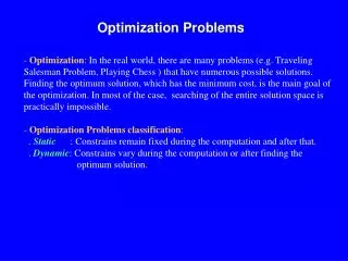
2. Computational complexity of discrete optimization problems • In terms of complexity of solution methods, discrete optimization problems can be divided into two classes: 1) Problems that have efficient algorithms for finding optimal solutions. 2) Problems that don’t have such efficient algorithms. • The first class problems (Minimum Spanning Tree Problem, Maximum Flow Problem, etc.) will be considered in the second half of this class. • Most discrete optimization problems are in the second class.

3. Efficiency of Algorithms • Two main issues related to the efficiency of algorithms:  Speed of algorithm  Efficient memory allocation • We will focus on the speed of algorithms. The speed of an algorithm (running time) is determined by the number of elementary operations: addition, subtraction, multiplication, division, comparison. The number of elementary operations depends on  problem size  nature of input data

4. Analysis of Running Time • Running time of an algorithm is a function of input size. • Two kind of analyses of running time:  Worst-case running time analysis  Average-case running time analysis Most results in the analysis of algorithms concern the worst-case running time.

5. Efficiency of Algorithms: Example • Recall the Traveling Salesman Problem (TSP): There are n cities. The salesman  starts his tour from City 1,  visits each of the cities exactly once,  and returns to City 1. For each pair of cities i, j there is a cost cijassociated with traveling from City i to City j . • Goal: Find a minimum-cost tour.

6. “Exhaustive enumeration” algorithm • One way of solving the problem is by an algorithm which is based on exhaustive enumeration (brute force): 1) Compute the costs of all possible tours; 2)Choose the tour with minimum cost. • What is the running time of this algorithm? 1)  The number of possible tours is (n-1)!  The cost of each tour is the sum of n individual costs  requires n-1 additions.  Thus, computing the costs of all possible tours requires (n-1)∙(n-1)! elementary operations. 2) Choosing the tour with minimum cost requires (n-1)!-1 comparisons. Summarizing, (n-1)∙(n-1)! + (n-1)! -1 = n! -1 elementary operations are needed for implementing the algorithm.

7. Efficiency of the “Exhaustive enumeration” algorithm • Is the “exhaustive enumeration” algorithm efficient? Assume that each elementary operation can be done in 1 nanosecond = 10-9 seconds. Then the running time:

8. “Nearest neighbor” algorithm • Consider another method for solving the TSP, the “Nearest neighbor” algorithm: In every iteration (except the last one) go to the closest city not visited yet. • What is the running time of this algorithm?  In each iteration we choose one of the n cities; so there are n iterations.  In each iteration, we need at most n comparisons to choose the next city. Thus, the total number of elementary operations is at most n2.

9. Efficiency of the “Nearest Neighbor” algorithm Compare the running times of “Nearest neighbor” and “Exhaustive enumeration” algorithms: Note: The “Nearest Neighbor” algorithm might not return an optimal solution.

10. Order of an Algorithm • Definition: Let A be an algorithm. Let w(n) be the maximum number of elementary operations required to execute A for all possible input sets of size n. If w(n) isO(f(n)) , we say that A has a (worst case) order of f(n) . • Ex.:Suppose the maximum number of operations needed to execute algorithm A is 5n2+3n+7 . Then A has an order of n2 .

11. Time comparisons of the most common algorithm orders

12. Polynomial-time algorithms and NP-hard problems • Definition: An algorithm is called polynomial-time if it has an order of f(n)=nk for some constant k. • Polynomial-time algorithms are considered efficient. (In practice, k>3 is not so good; but most known polynomial-time algorithms are for smaller k’s). • For Class 1 discrete optimization problems, there arepolynomial-time algorithms for solving the problems optimally. • For Class 2discrete optimization problems • No polynomial-time algorithm is known; • And more likely there is no one. • Class 2 problems are known as NP-hard problems. • How to solve NP-hard problems? (Next handout)