Download
1 / 41
420 likes | 617 Vues
Introduction to Macromolecular X-ray Crystallography Biochem 300 Borden Lacy. Print and online resources: Introduction to Macromolecular X-ray Crystallography , by Alexander McPherson Crystallography Made Crystal Clear , by Gale Rhodes http://www.usm.maine.edu/~rhodes/CMCC/index.html

E N D
Introduction to Macromolecular X-ray Crystallography Biochem 300 Borden Lacy Print and online resources: Introduction to Macromolecular X-ray Crystallography, by Alexander McPherson Crystallography Made Crystal Clear, by Gale Rhodes http://www.usm.maine.edu/~rhodes/CMCC/index.html http://ruppweb.dyndns.org/Xray/101index.html Online tutorial with interactive applets and quizzes. http://www.ysbl.york.ac.uk/~cowtan/fourier/fourier.html Nice pictures demonstrating Fourier transforms http://ucxray.berkeley.edu/~jamesh/movies/ Cool movies demonstrating key points about diffraction, resolution, data quality, and refinement. http://www-structmed.cimr.cam.ac.uk/course.html Notes from a macromolecular crystallography course taught in Cambridge
Overview of X-ray Crystallography Crystal -> Diffraction pattern -> Electron density -> Model Resolution, Fourier transforms, the ‘phase problem’, B-factors, R-factors, R-free …
Diffraction: The interference caused by an object in the path of waves (sound, water, light, radio, electrons, neutron..) Observable when object size similar to wavelength. Object Visible light: 400-700 nm X-rays: 0.1-0.2 nm, 1-2 Å
Can we image a molecule with X-rays? Not currently. 1) We do not have a lens to focus X-rays. Measure the direction and strength of the diffracted X-rays and calculate the image mathematically. 2) The X-ray scattering from a single molecule is weak. Amplify the signal with a crystal - an array of ordered molecules in identical orientations.
The wave nature of light l f(x) = Fcos2π(ux + a) f(x) = Fsin2π(ux + a) x F = amplitude u = frequency a = phase ul=c f(x) = cos 2πx f(x) = 3cos2πx f(x) = cos2π(3x) f(x) = cos2π(x + 1/4)
Interference of two waves Wave 1 + Wave 2 Wave 1 Wave 2 In-phase Out -of-phase
Bragg’s Law Sin q = AB/d AB = d sin q AB + BC = 2d sin q nl = 2d sin q
The intensity of each spot contains information about the entire molecule. The spacing of the spots is due to the size and symmetry of your lattice. Practically: Assign a coordinate (h, k, l) and intensity (I) to every spot in the diffraction pattern— Index and Integrate. Ihkl , shkl Diffraction pattern
Fourier transform: F(h)= ∫ f(x)e2πi(hx)dx where units of h are reciprocals of the units of x Reversible! f(x)= ∫ F(h)e-2πi(hx)dh
Calculating an electron density function from the diffraction pattern F(h) = Fcos2π(uh+ a) F(h) = Fsin2π(uh + a) r(x) = ∫ F(h)e-2πi(hx)dh F = amplitude u = frequency a = phase Experimental measurements: Ihkl, shkl Fhkl ~ √Ihkl
Overcoming the Phase Problem Heavy Atom Methods (Isomorphous Replacement) Anomalous Scattering Methods Molecular Replacement Methods Direct Methods
Heavy Atom Methods (Isomorphous Replacement) The unknown phase of a wave of measurable amplitude can be determined by ‘beating’ it against a reference wave of known phase and amplitude. Combined Wave Unknown Reference
Generation of a reference wave: Max Perutz showed ~1950 that a reference wave could be created through the binding of heavy atoms. Heavy atoms are electron-rich. If you can specifically incorporate a heavy atom into your crystal without destroying it, you can use the resulting scatter as your reference wave. Crystals are ~50% solvent. Reactive heavy atom compounds can enter by diffusion. Derivatized crystals need to be isomorphous to the native.
Native Fnat Heavy atom derivative Fderiv
Heavy Atom Methods (Isomorphous Replacement) The unknown phase of a wave of measurable amplitude can be determined by ‘beating’ it against a reference wave of known phase and amplitude. FPH FP FH and aH Can use the reference wave to infer aP. Will be either of two possibilities. To distinguish you need a second reference wave. Therefore, the technique is referred to as Multiple Isomorphous Replacement (MIR).
Overcoming the Phase Problem Heavy Atom Methods (Isomorphous Replacement) Anomalous Scattering Methods Molecular Replacement Methods Direct Methods
Anomalous scattering Incident X-rays can resonate with atomic electrons to result in absorption and re-emission of X-rays. Results in measurable differences in amplitude Fhkl ≠ F-h-k-l
Advances for anomalous scattering methods Use of synchrotron radiation allows one to ‘tune’ the wavelength of the X-ray beam to the absorption edge of the heavy atom. Incorporation of seleno-methionine into protein crystals.
Anomalous scattering/dispersion in practice Anomalous differences can improve the phases in a MIR experiment (MIRAS) or resolve the phase ambiguity from a single derivative allowing for SIRAS. Measuring anomalous differences at 2 or more wavelengths around the absorption edge: Multiple-wavelength anomalousdispersion (MAD). Advantage: All data can be collected from a single crystal. Single-wavelength anomalous dispersion (SAD) methods can work if additional phase information can be obtained from density modification.
Overcoming the Phase Problem Heavy Atom Methods (Isomorphous Replacement) Anomalous Scattering Methods Molecular Replacement Methods Direct Methods
Molecular Replacement If a model of your molecule (or a structural homolog) exists, initial phases can be calculated by putting the known model into the unit cell of your new molecule. 1- Compute the diffraction pattern for your model. 2- Use Patterson methods to compare the calculated and measured diffraction patterns. 3- Use the rotational and translational relationships to orient the model in your unit cell. 4- Use the coordinates to calculate phases for the measured amplitudes. 5- Cycles of model building and refinement to remove phase bias.
Direct Methods Ab initio methods for solving the phase problem either by finding mathematical relationships among certain phase combinations or by generating phases at random. Typically requires high resolution (~1 Å) and a small number of atoms. Can be helpful in locating large numbers of seleno-methionines for a MAD/SAD experiment.
Overcoming the Phase Problem Heavy Atom Methods (Isomorphous Replacement) Anomalous Scattering Methods Molecular Replacement Methods Direct Methods FT F = amplitude u = frequency a = phase r(x,y,z) electron density
Are phases important? Duck intensities and cat phases
Does molecular replacement introduce model bias? Cat intensities with Manx phases
An iterative cycle of phase improvement Building Refinement Solvent flattening NCS averaging
Model building Interactive graphics programs allow for the creation of a ‘PDB’ file. Atom type, x, y, z, Occupancy, B-factor
The PDB File: ATOM 1 N GLU A 27 41.211 44.533 94.570 1.00 85.98 ATOM 2 CA GLU A 27 42.250 44.748 95.621 1.00 86.10 ATOM 3 C GLU A 27 42.601 43.408 96.271 1.00 85.99 ATOM 4 O GLU A 27 43.691 42.865 96.065 1.00 85.71 ATOM 5 CB GLU A 27 41.725 45.720 96.687 1.00 86.36 ATOM 6 CG GLU A 27 42.804 46.349 97.563 1.00 86.44 ATOM 7 CD GLU A 27 43.628 47.387 96.817 1.00 86.98 ATOM 8 OE1 GLU A 27 44.194 47.051 95.754 1.00 87.40 ATOM 9 OE2 GLU A 27 43.713 48.540 97.296 1.00 87.02 ATOM 10 N ARG A 28 41.662 42.882 97.053 1.00 85.65 ATOM 11 CA ARG A 28 41.839 41.607 97.739 1.00 85.29 ATOM 12 C ARG A 28 41.380 40.458 96.835 1.00 85.31 ATOM 13 O ARG A 28 42.184 39.619 96.424 1.00 85.09 ATOM 14 CB ARG A 28 41.035 41.607 99.045 1.00 84.62 ATOM 15 CG ARG A 28 39.564 41.944 98.851 1.00 84.07 ATOM 16 CD ARG A 28 38.845 42.152 100.169 1.00 84.00 ATOM 17 NE ARG A 28 37.423 42.439 99.980 1.00 84.27 ATOM 18 CZ ARG A 28 36.945 43.413 99.208 1.00 84.53 ATOM 19 NH1 ARG A 28 37.771 44.208 98.537 1.00 83.83 ATOM 20 NH2 ARG A 28 35.634 43.598 99.111 1.00 84.38 . . .
Occupancy What fraction of the molecules have an atom at this x,y,z position? B-factor How much does the atom oscillate around the x,y,z position? Can refine for the whole molecule, individual sidechains, or individual atoms. With sufficient data anisotropic B-factors can be refined.
Refinement Least -squares refinement • = Swhkl (|Fo| - |Fc|)2hkl Apply constraints (ex. set occupancy = 1) and restraints (ex. specify a range of values for bond lengths and angles) Energetic refinements include restraints on conformational energies, H-bonds, etc. Refinement with molecular dynamics An energetic minimization in which the agreement between measured and calculated data is included as an energy term. Simulated annealing often increases the radius of convergence.
S||Fobs| - |Fcalc|| R = S|Fobs| Monitoring refinement Rfree: an R-factor calculated from a test set that has not been used in refinement.