Production Technology
Production Technology. Chapter 7. Introduction. Aim in this chapter Investigate purely technical relationship of combining inputs to produce outputs Presents a physical constraint on society’s ability to satisfy wants Classify factors going into production process

Production Technology
E N D
Presentation Transcript
Production Technology Chapter 7
Introduction • Aim in this chapter • Investigate purely technical relationship of combining inputs to produce outputs • Presents a physical constraint on society’s ability to satisfy wants • Classify factors going into production process • Derive a production function that establishes a relationship between production factors and a firm’s output • Discuss Law of Diminishing Marginal Returns and stages of production • Develop concept of isoquants • When two production factors are allowed to vary • Can substitute one factor for another • Measure of this ability is elasticity of substitution • Effect of proportional changes in all inputs is called returns to scale • Can classify production functions in terms of their elasticity of substitution and returns to scale attributes
Factors of Production • For economic modeling, factors of production are generally classified as • Capital • Durable manmade inputs • Are themselves produced goods • Labor • Time or service individuals put into production • Land • All natural resources (for example, water, oil, and climate) • Classification allows us to conceptualize simple cases first • Then extend analysis to higher dimensions that are more general (realistic)
Factors of Production • Time also enters into production process • Economists generally divide time into three periods, based on ability to vary inputs • Market period • All inputs are fixed • Short-run period • Some inputs are fixed and some are variable • Long-run period • All inputs are variable • In terms of actual time, market-period, short-run, and long-run intervals can vary considerably from one firm to another, • Depends on nature of a particular firm • Division of time into three periods is a simplification • With intertemporal substitution among stages • More general models incorporating numerous time stages are less restrictive in their assumptions • Called dynamic models
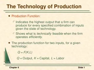
Production Functions • Firms are interested in turning inputs into outputs with the objective of maximizing profit • Formalized by a production function • q = ƒ(K, L, M) • Where q is output of a particular commodity • K is capital • L is labor • M is land or natural resources • For any possible combination of inputs, production function records maximum level of output that can be produced from that combination • In market period all inputs are fixed, so level of output cannot be varied
Production Functions • Denote K°, L°, and M° as the fixed level of capital, labor, and land • Production from these fixed inputs is fixed at q°, so • q° = ƒ(K°, L°, M°) • If capital and labor could be varied with only land fixed, then a short-run production function would be • q = ƒ(K, L, M°) • Now possible to vary output by changing either K or L • Or both K and L • In long run, all inputs could be varied, so only restriction on output is technology • Production function represents set of technically efficient production processes • Yields highest level of output for a given set of inputs
Production Functions • Generally, technical aspects of production do impose restrictions on profit • Assumptions (axioms) concerning these aspects are required for developing economic models • Two axioms generally underlie a production function • Monotonicity • Implies that if a firm can produce q with a certain level of inputs • Should be able to produce at least q if there exists more of every input • Assumes free disposal of inputs • Implies that all marginal products of the variable inputs are positive at their profit-maximizing level • Strict convexity • Analogous to Strict Convexity Axiom in consumer theory
Variations in One Input (Short Run) Marginal Product • Marginal product (MP) of variable input • Change in output, Δq, resulting from a unit change of the variable input • Holding all other inputs constant • If capital is variable input, then marginal product of capital is • Alternatively, if labor is variable input, then marginal product of labor is • MP is analogous to concept of marginal utility except that MP is a cardinal number measured on the ratio scale • Not an ordinal number
Variations in One Input (Short Run) Marginal Product • Distances between any levels of MP are of a known size measured in physical quantities • Bushels, crates, pounds, etc. • Consider following cubic production function with labor as variable input • q = 6L2 – ⅓L3 • Marginal product of labor is • MPL = 12L – L2 • Graph of production function and MPL is provided in Figure 7.1
Variations in One Input (Short Run) Marginal Product • At first, for low levels of labor, total product (TP) is increasing at an increasing rate • Slope of TP or MPL is rising • At point of inflection, slope is at its maximum • MPL is also at a maximum • To right of maximum MPL, TP is still increasing • But at a decreasing rate • MPL is positive, but falling • At maximum TP, slope of TP curve is zero • Corresponding to MPL = 0 • When TP is falling, MPL is negative • According to Monotonicity Axiom, given free disposal, a firm will not operate in negative range of MPL • Generally assumed that MPL ≥ 0
Average Product • According to U.S. Department of Labor, output per hour of labor for nonfarm business increased at an annual rate of 2.1% from 1991 to 2000 • Measure of productivity is measured in physical quantities • Called average product (AP) of an input • Defined, for labor, as • APL = q/L • In general, average product (AP) is output (TP) divided by input • In Figure 7.1, APL at first increases, reaches a maximum, then declines • Productivity of labor, as measured by APL, changes as additional workers are employed • Results from short-run condition that all other inputs remain fixed • At first, with a relatively small number of workers for a large amount of other inputs • Adding an additional worker increases productivity of all workers • APL increases • However, a point is reached where labor is no longer relatively limited compared with fixed inputs • An additional worker will result in APL declining
Average Product • Graphically, we can determine APL from TP curve by considering a line (cord) through origin • Slope of a cord through origin is TP divided by labor • Since APL is defined as TP divided by labor • Slope of a cord through origin is APL at a level of labor where cord intersects TP • As number of workers increases, at first cord shifts upward and slope of the cord increases • Resulting in increased APL • Can continue to shift cord upward and it will continue to intersect TP curve until it finally is tangent to TP curve • At this point, APL is at its maximum
Law of Diminishing Marginal Returns and Stages of Production • A firm’s costs will depend on • Prices it pays for inputs • Technology of combining inputs into output • In short run firm can change its output by adding variable inputs to fixed inputs • Output may at first increase at an increasing rate • However, given a constant amount of fixed inputs, output will at some point increase at a decreasing rate • Occurs because at first variable input is limited compared with fixed input • As additional workers are added, productivity remains very high • Output, or TP, increases at an increasing rate • However, as more of variable input is added, it is no longer as limited • Eventually, TP will still be increasing, but at a decreasing rate • MPL will still be positive, but declining • CalledLaw of Diminishing Marginal Returns (or just diminishing returns)
Law of Diminishing Marginal Returns and Stages of Production • As indicated in Figure 7.1, diminishing marginal returns starts at point A • MPL is at a maximum • To the left of point A there are increasing returns and at point A constant returns exist • Between points A and B, where MPL is declining, diminishing marginal returns exist • To the right of point B, marginal productivity is both diminishing and negative (MPL < 0), which violates Monotonicity Axiom • TP curve will at some point increase only at a decreasing rate (concave) due to Law of Diminishing Marginal Returns • Some production functions may not exhibit increasing returns at first • In fact no firm with a profit-maximizing objective will operate in area of increasing returns or negative returns • Production functions generally will only be concave • With diminishing marginal returns throughout production process • Depicted in Figure 7.2
Figure 7.2 Production function with diminishing marginal returns throughout
Law of Diminishing Marginal Returns and Stages of Production • In Figure 7.2 MPL and APL decline throughout • Cobb-Douglas production function can also only exhibit diminishing marginal returns throughout production process • Can characterize production where all marginal products are positive • Useful for representing firms’ technology constraints • Given that profit-maximizing firms will only operate in area of diminishing marginal returns where all marginal products are positive • Illustrated in Figure 7.3 for a variable level of labor
Figure 7.3 Cobb- Douglas production function with labor as the only variable input
Relationship of Marginal Product to Average Product • In area of diminishing marginal returns, marginal product can intersect with average product • As indicated in Figure 7.1, this intersection of MPL and APL occurs where APL is at a maximum • If addition to total, marginal unit, is greater (less) [equal to] than overall average • Average will rise (fall) [neither rise nor fall] • Taking derivative of average results in relationship between marginal product and average product • Marginal product is average product plus an adjustment factor (APL/L)L • If slope of APL is zero (rising) [falling] • Adjustment factor is zero (> 0) [< 0] • MPL = APL (MPL > APL) [MPL < APL]
Output Elasticity • Another important relation between an average and marginal product is output elasticity • Measures how responsive output is to a change in an input • For example, output elasticity of labor, denoted L, is defined as proportionate rate of change in q with respect to L • Given production function • q = ƒ(K, L) • Output elasticity of labor is • L = (ln q)/ (ln L) = (q/L)(L/q) = MPL/APL • When MPL > APL, L > 1; when 0 < MPL < APL, 0 < L < 1; and when MPL < 0, L < 1 • Illustrated in Figure 7.1
Stages of Production • Firm must determine profit-maximizing amount of an available input it should employ • Use technology of production to determine at what stage of production to add a variable input, say, labor • Exact profit-maximizing level of labor within this stage depends on • Cost of labor • Price received for the firm’s output • Specifically, we divide short-run production function into three stages of production
Stages of Production • Stage I includes area of increasing returns and extends up to point where average product reaches a maximum • Illustrated in Figure 7.1 • Includes a portion of marginal product curve that is declining • Marginal product is greater than average product, so average product is rising • As long as average product is rising, firm will add variable inputs • Fixed inputs are present in uneconomically large proportion relative to variable input • Variable input is limited relative to fixed inputs • Rational profit-maximizing producer would never operate in Stage I of production • Firm would not produce in short run • Would produce by using fewer units of fixed inputs in long run • Fixed inputs become variable • Reduction of fixed inputs would result in entire set of product curves shifting leftward • Results in Stage I ending at a lower level of output • Illustrated in Figure 7.4
Figure 7.4 Shifts in stages of production with a reduction in the level of fixed inputs
Stages of Production • Rational producer will also not operate in Stage III of production • Range of negative marginal product for variable input • In Stage III, TP is actually declining as more of the variable input is added • Figures 7.1, 7.2, and 7.4 illustrate Stage III • Additional units of the variable input Stage III actually cause a decline in total output • Even if units of variable input were free, a rational producer would not employ them beyond the point of zero marginal product • In Stage III, variable input is combined with fixed input in uneconomically large proportions • Indeed, point of zero MP, for variable input, is called intensive margin • Point of maximum AP of variable input is called extensive margin • A firm will operate between extensive and intensive margins • Stage II of production • Both AP and MP of variable input are positive but declining • Output elasticity is between 0 and 1 • In contrast, output elasticity for variable input is < 0 in Stage III and > 1 in Stage I
Two Variable Inputs • Assumed a different combination of, say two, inputs will produce same level of output • For example, in manufacturing microwave ovens, greater use of plastics may be substituted for a reduction in metal use • Indifference curves represent a consumer’s preferences for different combinations of two goods with utility remaining constant • In production theory isoquants represent different input combinations that may be used to produce a specified level of output • Iso means equal and quant stands for quantity • An isoquant is a locus of points representing same level of output or equal quantity • For movements along an isoquant • Level of output remains constant • Input ratio changes continuously • Isoquants are the same concept as indifference mapping • Equal utility along same indifference curve replaced by equal output level along same isoquant • Figure 7.5 represents a possible production function for two inputs
Figure 7.5 Isoquant map for two variable inputs, capital, K, and labor, L
Marginal Rate of Technical Substitution (MRTS) • In Figure 7.5, isoquants are drawn with a negative slope • Based on assumption that substituting one input for another can result in output not changing • A measure for this substitution is marginal rate of technical substitution (MRTS) • Defined as negative of slope of an isoquant • Measures how easy it is to substitute one input for another holding output constant • Similar to concept of MRS in consumer theory • MRTS measures reduction in one input per unit increase in the other that is just sufficient to maintain a constant level of output
Convex and Negatively Sloping Isoquants • Can establish underlying assumptions of negatively sloped and convex-to-the-origin isoquant by developing relationship between MRTS and MPs • MRTS (K for L) = MPL ÷ MPK • Take total derivative of production function, q = ƒ(K, L) • dq = MPLdL + MPKdK • Along an isoquant dq = 0, output is constant • Thus MPLdL = -MPKdK • Solving for the negative of the slope of the isoquant yields • Along an isoquant, gain in output from increasing L slightly is exactly balanced by loss in output from a suitable decrease in K • For isoquants to be negatively sloped, both MPL and MPK must be positive • Ridgelines trace out boundary in isoquant map where marginal products are positive • See Figure 7.6 • Ridgelines are isoclines (equal slopes) where MRTS is either zero or undefined for different levels of output
Convex and Negatively Sloping Isoquants • MRTS results in isoquants drawn strictly convex to origin • Result is analogous to relationship between MRS and strictly convex indifference curves • For high ratios of K to L MRTS is large • Indicating that a great deal of capital can be given up if one more unit of labor becomes available • Assumption of strictly convex isoquants is related to Law of Diminishing Marginal Returns • Given MRTS(K for L) = MPL/MPK • Movement from A to B in Figure 7.6 results in an increase in labor • Corresponding decrease in MPL • Decrease in capital with a corresponding increase in MPK • A firm will always operate in Stage II of production • Characterized by diminishing marginal returns • Stage II of production, for both the variable inputs, is represented by strictly convex isoquants • In Figure 7.6, a rational producer will only operate somewhere between points D and C
Stages of Production in the Isoquant Map • Can illustrate stages of production in isoquant map by fixing one of the inputs • A situation where capital is fixed at some level is indicated by horizontal line at A in Figure 7.7 • In short run, firm must operate somewhere on this line • At Stage I, labor input is small relative to fixed level of capital • Marginal product of capital and MRTS are negative • Isoquants have positive slopes • At point B, MRTS is undefined, MPK is zero, and APL equals MPL • This is demarcation between Stages I and II of production • In Stage II of production, all isoquants are strictly convex and have negative slopes • At point C, marginal product of labor is zero • Corresponds to line of demarcation between Stages II and III
Classifying Production Functions • Production functions represent tangible (measurable) productive processes • Economists pay more attention to actual form of these functions than to form of utility functions • Resulted in classification of production functions in terms of returns to scale and substitution possibilities • Empirical estimates of actual production functions • For some production processes it may be extremely difficult if not impossible to substitute one input for another
Returns to Scale • Measure how output responds to increases or decreases in all inputs together • Long-run concept since all inputs can vary • For example, if all inputs are doubled, returns to scale determine whether output will double, less than double, or more than double • In many cases, it is difficult to change some inputs at will and increase inputs proportionally • Firms do attempt to control as much of environmental conditions as feasible • Examples in agriculture include greenhouses or pesticides • Assuming it is possible to proportionally change all inputs, a production function can exhibit constant, decreasing, or increasing returns to scale across different output ranges • However, it is generally assumed, for simplicity, production functions only exhibit either constant, decreasing, or increasing returns to scale
Returns to Scale • Specifically, given production function • q= ƒ(K, L) • A explicit definition of constant returns to scale is • ƒ(K, L) = ƒ (K, L) = q, for any > 0 • If all inputs are multiplied by some positive constant , output is multiplied by that constant also • If production function is homogeneous • Constant returns to scale production function is homogeneous of degree 1 or linear homogeneous in all inputs • Isoquants are radial blowups and equally spaced as output expands (Figure 7.8)
Returns to Scale • Decreasing returns to scale exists if output is increased proportionally less than all inputs • ƒ(K, L) < ƒ(K, L) = q • Increasing returns to scale exists if output increases more than proportional increase in inputs • ƒ(K, L) > ƒ(K, L) = q
Determinants of Returns to Scale • Adam Smith established that returns to scale is result of two forces • Division of labor • An increase in all inputs increases division of labor and results in increased efficiency • Production might more than double • Managerial difficulties • Result in decreased efficiency • Production might not double • Early 20th century concept of assembly-line mass production is based on division of labor • Each worker has a specialized task to perform for each product being assembled • Worker becomes very skilled at this task • Increases productivity • Example: Henry Ford experienced increasing returns to scale in automobile manufacturing
Determinants of Returns to Scale • One cause of managerial difficulties in mass production is required stockpiling of parts and supplies • Inventory control must be maintained, where an accounting of parts is required • Results in a significant amount of inputs allocated to storage and accounting of inventories • Results in decreasing returns to scale • Just-in-time delivery systems are helping to mitigate these factors • One problem with just-in-time production • Increased vulnerability of firms to supply disruptions • Without a stockpile of parts, such disruptions could shut down production fairly quickly
Determinants of Returns to Scale • Postindustrial manufacturing is shifting away from mass production of a standardized product and evolving toward mass customization • Called agile manufacturing • Results in increasing returns to scale
Determinants of Returns to Scale • As a firm increases in size by increasing all inputs, another possible cause of decreasing returns to scale is • Allocation of inputs for environmental and local service projects • As a firm employs more inputs and increases output, it becomes increasingly more exposed to public concerns associated with its production practices • To enhance and maintain goodwill within its community, firm will allocate additional inputs for environmental and local service projects • Contributes to decreasing returns to scale
Returns to Scale and Stages of Production • Determine relationship between returns to scale and stages of production by assuming a linear homogeneous production function (homogeneous of degree 1) • Implies a constant returns to scale production function • Applying Euler’s Theorem to production function q = ƒ(K, L) we obtain • q = L(MPL) + K(MPK) • Dividing by L gives • APL = MPL + (K/L)MPK • Solving for MPK yields • MPK = (L/K)(APL – MPL)
Returns to Scale and Stages of Production • Assuming constant returns to scale, we define stages of production as • Stage I • MPL > APL > 0, MPK < 0 • Stage II • APL > MPL > 0, APK > MPK > 0 • Stage III • MPL < 0, MPK > APK > 0 • Stages I and III are symmetric for a constant returns to scale production function • Given Monotonicity Axiom, only relevant region for production is Stage II
Elasticity of Substitution • A firm may compensate for a decrease in use of one input by an increase in use of another • Heinrich von Thunen collected evidence from his farm in Germany that suggested ability of one input to compensate for another was significant • Postulated principle of substitutability • Possible to produce a constant output level with a variety of input combinations • Principle of substitutability is not an economic law • There are production functions for which inputs are not substitutable • However, for those functions where inputs are substitutable • Degree that inputs can be substituted for one another is an important technical relationship for producers • Production functions may also be classified in terms of elasticity of substitution • Measures how easy it is to substitute one input for another • Determines shape of a single isoquant
Elasticity of Substitution • In Figure 7.9 consider a movement from A to B • Results in capital/labor ratio (K/L) decreasing • Profit-maximizing firm is interested in determining a measure of ease in which it can substitute K for L • If MRTS does not change at all for changes in K/L, the two inputs are perfect substitutes • If MRTS changes rapidly for small changes in K/L, substitution is difficult • If there is an infinite change in the MRTS for small changes in K/L (called fixed proportions), substitution is not possible • A scale-free measure of this responsiveness is elasticity of substitution
Elasticity of Substitution • Defined as percentage change in K/L divided by percentage change in MRTS • Along a strictly convex isoquant, K/L and MRTS move in same direction • Elasticity of substitution is positive • In Figure 7.9, a movement from A to B results in both K/L and MRTS declining • Relative magnitude of this change is measured by elasticity of substitution • If it is high, MRTS will not change much relative to K/L and the isoquant will be less curved (less strictly convex) • A low elasticity of substitution gives rather sharply curved isoquants • Possible for the elasticity of substitution to vary for movements along an isoquant and as the scale of production changes • However, frequently elasticity of substitution is assumed constant
Elasticity of Substitution: Perfect-Substitute • = , a perfect-substitute technology • Analogous to perfect substitutes in consumer theory • A production function representing this technology exhibits constant returns to scale • ƒ(K, L) = aK + bL = (aK + bL) = ƒ(K, L) • All isoquants for this production function are parallel straight lines with slopes = -b/a • See Figure 7.10
Figure 7.10 Elasticity of substitution for perfect-substitute technologies