Download
1 / 64
670 likes | 843 Vues
Advance Gamma Tracking Array AGATA Dino Bazzacco INFN Padova. Part 1: Review of AGATA Part 2: Data Processing. EGAN school 2011, December 5 - 9, 2011, Liverpool. Architecture of the system. Local Level : where the individual detectors don’t know of each other.

E N D
Advance Gamma Tracking Array AGATA Dino BazzaccoINFN Padova Part 1: Review of AGATA Part 2: Data Processing EGAN school 2011, December 5 - 9, 2011, Liverpool
Architecture of the system • Local Level : where the individual detectors don’t know of each other. • Electronics and computing follow a model with minimum coupling among the individual elements (detectors), which are operated independently as long as possible • Electronics is almost completely digital, operated on the same 100 MHz clock • Data processing (in the electronics and in the front-end computers) is the same for all detectors and proceeds in parallel • Every chunk of data produced is tagged with a time stamp that gives the absolute time (with a precision of 10 ns) since the last startup of the system. (with 48 bits the roll around takes place every 32.5 days) • Global Level : where the detectors do know of each other • By means of the real time trigger, which reduce the data rate by selecting the class of interesting events • Via the event builder and merger that assemble the event fragments (including the ancillaries) into complete events that are further processed • In the tracking and in the Physical analysis stages • The fact that 3 (and 2 at GSI) crystals are packed in clusters does not produce any correlation in the data processing (not so for the Detector Support System, but this is not relevant here)
GL Trigger Detector preamp. Digitisers Ancillary Clock 100 MHz T-Stamp Up to 180detectors Ancillary Core + 36 seg. PreProcessing & PSA Preprocessing EventBuilder Control, Storage… Tracking Ancillary Structure of Electronics and DAQ Analogue Synchronous Buffered Other detectors • interface to GTS via mezzanine • merge time-stamped data into event builder (merger)
AGATA Data Processing Digitisersin the experimental hall Digital proc. electronicsin the users area Computer farm in the computing room LAN to the disk servers 80 m long optical fibers 20 m long optical fibers 10 m long MDR cables • One digitizer per crystal:- core module with 1 core board (clock + 2 cores) • 2 segment boards (A B ) • segment module with 4 segment boards (C D E F ) 2 ATCA carriers per crystal: - Master with 1 GTS mezzanine 3 proc. mezzanines (Core A B) - Slave with 4 proc. mezzanines (C D E F) • 1 pizza-box per crystal: • Readout and save orig. data • Pre-processing of events • PSA10 pizza-boxes for • Event Builder and Merger • Ancillary and Tracking • 120 TB of storage + • Archiving on Grid T1 6 channels processing mezzanine
GL-Trigger GL-Trigger to reduce event rate to whatever value PSA will be able to manage Data rates in AGATA Demonstrator50 kHz singles 1 kHz triggered SEGMENT Pre-processing save 1 ms of pulse rise time 200 MB/s 100 Ms/s 14 bits + - Energy+· · · ADC 7.6 GB/s ~ 200 B/channel ~ 2 kB/s/channel LL-Trigger (CC) DETECTOR E, t, x, y, z,... ~1 ms/event Pulse Shape Analysis 200 B/event 0.2 MB/s/det. 36+2 9296 B/event 10 MB/s Compression factor ~2 5 MB/s/det. raw data to disk GLOBAL + ~1 MB/s from ancillary detectors, when used < 5 MB/s Event Builder g-ray Tracking HL-Trigger, Storage On Line Analysis 15*0.2 3 MB/s 180*0.2 36 MB/s (Full AGATA) 40 MB/s Saving the original data produces ~5 ÷ 30 TB / experiment Our disk server (100 TB) is always almost full data archived to the GRID
GTS : the system coordinatorAll detectors operated on the same 100 MHz clock Downwards 100 MHz clock + 48 bit Timestamp (updated every 16 clock cycles) Upwards trigger requests, consisting of address (8 bit) and timestamp (16 bit) max request rate 10 MHz total, 1 MHz/detector Downwards validations/rejections, consisting or request + event number (24 bit) M.Bellato , Agata Week Darmstadt - 6-9 September 2011
GTS Tree with theFully Digital Trigger Processor GTS tree to: - Distribute the 100 MHz clock- Collect the trigger requests (i.e. 16-bit time stamp and address of the requesting node)- Return validations or rejections messages to the requesting node Max 1 MHz trigger requests/node Built out of GTS mezzanines - Runs on an evaluation board with a VIRTEX5 FPGA - Partitions and sum buses implemented in VHDL - 2nd level logic is implemented in C and runs in the PPC - Uses idle-messages to timeout non-participating nodes - Present version has 48 inputs and 4 partitions - Each partition has 4 multiplicity thresholds - The two partitions can be operated in coincidence P1 with the Ge crystals Trig1 P1 >=1 & P2 = 1 P2 with the ancillary Trig2 P1 >=2 Handles max 100 kHz of coincidences (limited by PPC) The “3 to 1” structure can beextended up to 3 levels 9 triple clusters or 8 triple clusters + 3 ancillaries Marco Bellato, LucianoBerti, JoëlChavas
Available Triggers • multiplicity • up to 4 partitions(P), each one with 4 multiplicity thresholds • often used with 1 partition containing the 15 Ge detectors • digital version of the classical multiplicity sum bus • ancillary • P1(Ge) AND P2(Ancillary) coincidence condition is a window on the timestamps • ancillary2 • (P1 AND P2) OR (P2 AND NOT P1)(e.g. validate PRISMA even if thereis no gamma coincidence) • Service triggers • validate_all • reject_all
Digitizers • 100 MS/s • max frequency correctly handled is 50 MHz (Nyquist) • 14 bits • Effective number of bits is ~12.5 (SNR ~75 db) • 2 cores and 36 segments (in 6 boards) • Core 2 ranges 5, 20 MeV nominal • Segments either high or low gain • The digitized samples are serialized and transmitted via optical fibre (1/channel) to the preprocessing electronics. Transmission rate is 2 Gbit/s on each of the 38 fibres. • Power consumption 240 W • Weight 35 kg
Beware of aliasing! Sampling theorem: analogue input signals limited to a bandwidthfBW can be reproduced from their samples with no loss of informationif they sampled at a frequency fs≥ 2fBW Nyquist frequency At 100 Ms/s, the preamplifier signals must be filtered, at the input of the,the digitizer to remove frequencies above 50 MHz (in practice above ~20 MHz)
AGATA Digitisers As the digitizers just digitize and transmit the sample, they operate very smoothly, need to be power-cycled very rarely, which is good for the gain stability of the signals.
Range of digitizers 1 5B 3B 2B 4B 1B 5G 3G 2G 4G 1G 5R 3R 2R 4R 1R Some cores and segments saturate below 3 MeV on the high-gain range Gain in the digitizers should be reduced by ~30% test5atc_110603/run_000
Range of Digitizers Values derived from the energy calibration coefficients , with offsets adjusted to have the “zero”of preamp signals at ¼ of the conversion range
Range of digitizers 2 Operation at high counting rates 1 ms 1R CC high gain 1R CC low gain 1R B1 (low gain) CC ~30 kHz segment B1 ~7 kHz
Preprocessing Electronics • Fully digital, processing 38 channels in parallel for each crystal. • Receives the continuous stream of samples from the digitizers. • Generates the energy by means of a trapezoidal shaper • Generates the local trigger on the core (CC) signal by Leading Edge Discriminator (or CFD) • Takes a snap shot of 1 ms (100 samples) on all 38 channels • Sends validated events to the front-end computers • For 1 crystals: 2 ATCA carrier boards, 7 processing mezzanines and 1 GTS node.
Signal Processing in the electronics • Noise and disturbances in the signals • Effective band width of the signals • Deconvolution of the main pole • Deconvolution of 2nd order effects in detector/preamp chain (multiple poles) • Triangular (trapezoidal) shaping • Adaptive shaping for high counting rates • More sophisticated BLR • Treatment of saturated signals by ToT • …
Convolution and Correlation Signal processing blocks can be often described as linear (and time invariant) systems that act on an the input to produce an output. • Convolution: how a linear system acts on the input to produce the output • Correlation: evidences similarity of two signals • Autocorrelation: short and long term correlations in a signal h[n] is the transfer function of the system
Transforms • Mapping of one space to another (dual) in order to simplify and/or speed-up operations that are difficult and/or slow in the original one space. • Fourier Transform time ↔ frequency • Analysis of noise, detector response function, action of filters and shapers • Laplace Transform time ↔ s • Solving differential equations • Z Transform sample number ↔ z • Solving difference equations and expressing in an analytical way filters and shapers • Common and useful properties • Linearity T(a·f(t) + b·g(t)) = a·T(f(t)) + b·T(g(t)) • Derivation D(f(t)) = s·T(f(t)) + initial condition • Integration I(f(t)) = T(f(t))/s • Convolution T(f(t)g(t)) = T(f(t)) ·T(g(t)) • In general the original and transformed variables are complex .In Signal Processing the original data is almost always real and the transformed variable is often also real (e.g. power spectra with allphases set to zero so that only the amplitude is of interest)
Fourier Transform(s) The Scientist and Engineer's Guide to Digital Signal Processing By Steven W. Smith www.dspguide.com/index.htm
Discrete Fourier Transformof real signals dspguide Forward decomposition Inverse synthesis N real signals mapped to N coefficients ( N+2, but 2 are identically zero: sin[0], sin[N/2]) Vector representation (cos,sin) useful for calculations Polar representation (magnitude, phase) used for human inspection For large N, calculated using the Fast Fourier Transfor (FFT) algorithm
Useful theorems • Parseval: correspondence between time and frequencypower spectra • Wiener-Kintchine: the autocorrelation function of a signal is the Inverse Fourier Transform of its the power spectral density S|xn|2 / N corresponds to the variance s2 if the “noise” spectra have <xn>=0 The integrated noise power of the DFT spectra is multiplied by 2 because we use only positive frequencies up to Nyquist (unilateral representations).
Noise spectrum from “empty” sampled signals Sampled signals of “noise” Averaged noise amplitude unsing only “empty” traces 100000 samples * 10 ns 1 ms frequency resolution 1 kHz
Noise spectra of ATC1 Amplitude (kev/√Hz) Frequency kHz (2010-03-18 after improving grounding)
Autocorrelation of noise • Autocorrelation determined from the inverse of the noise density power spectrum, obtained by averaging “empty” traces • Autocorrelation enhances the evidence of periodic disturbances • Allows to determine the high frequency cut of the total preamplifier+digitizer transfer function
Repetitive disturbances Gaussian bursts Repetition 50 kHz High frequency 8 MHz
High frequency cut of spectrum Autocorrelation rotated to the centre; normalized to the maximum for the 4 channels CC t = 16 ns A4,A5 t = 30-35 ns as most of the other segments A1 t = 14 ns as A2 and A3 (preamplifier board not slowed down)
“Deconvolution” of Gesignals • Signals from Ge preamplifiers are, ideally, exponentials with only one decay constant • Task of the deconvolution is to remove the exponential to recover the original d(t) at the input of the preamplifier • Trapezoidal shaping is then just an integration followed by delayed subtraction followed by a moving average • In practice Trapezoidal shaping is the optimum shaping if the noise is white and the collection time (width of the “delta”) varies a lot as in the large volume semi-coax Ge AGATA detectors R • In practice the output exponential is produced in stages : • - RCF charge loop with decay constant t0~1 ms • - CR differentiation to reduce the decay constant to t1 ~50 ms • - P/Z cancellation to remove the undershoot and the long recovery (with t=t0) due to the differentiation of the first exponential. CF CI=CS+CP+CA vi(t) vo(t) A ii(t)=Q·δ(t)
Essentials of the z-transform • Development of shapers done using the z-transform formalism. • The most useful result is: if in the z domain the system function can be expressed as ratio of polynomials, in the time domain it is possible to realize it as a FIR or an IIR recursive filter with coefficients given by the coefficients of the polynomials. • We proceed in an informal way, assuming that the ROC exists and corresponds to one-sided casual signals • The relevant z-transform features are: z-domain time domain
Synthesis of Trapezoid by a cascade of filters Moving sum Moving average Other formulations and implementations A.Georgiev and W. Gast, IEEE Trans. Nucl. Sci., 40(1993)770 “Moving Window Deconvolution”V.T.Jordanov and G.F.Knoll, Nucl.Instr.Meth., A353(1994)261
Deconvolution and shaping: ideal exponential Flat topM=100 Any point of the flat-top is a good measure of the energy RisetimeK=1000
2011_week23 (R.Chapman, F.Haas) Segment A6 ~3 kHz Shaping 2.5-1-2.5 ms Life is more complicated for real signal Core (low gain) ~40 kHz Shaping 2.5-1-2.5 ms Base line not at zero and fluctuating. Need to use theBase Line Restorer (BLR), a time variant filter that averagesthe baseline when the trapezoid is below a given amplitude. Signal Amplitude = Value at flat-top – value of baseline
Base-line stabilisation • continuous (exponential) average of baseline • automatic detection of pulses based on variance • feed-back to deconvolution stage to bring baseline down to zero Upper part without feedback (as used at present) Lower part with feedback (used in the next electronics)
Adjustment of decay constant is critical for a good flat top 7700 Energy readout towards the end of flat top Readout time fixed by the trigger on CC t = 43.6 ms t = 46.4 ms 7600
Effect of shaping on noise Exponential with t=4600 samples Trapezoidal shaping 1900-100-1900 Total width 3900 Trapezoid 1000-1000-1000 + averaging 900 Flat top 100 Total width 3900
Amplitude keV/√(kHz) Fourier spectrum of noise for S001 CC frequency (kHz) Noise spectrum from DFT-1 Amplitude FWHM = 4.87*2.355 = 11.48 keV Sample number
Time domain convolution with the 2 transfer functions Quasi triangular Trapezoidal + average FWHM (quasi-triangular) = 0.559*2.355 = 1.32 keV FWHM (trap. + average) = 0.612*2.355 = 1.44 keV Frequency domain multiplication with the 2 transfer functions Original Shaped by quasi-triangular Shaped by trap. + average
Noise component of energy resolution from Integrated Power Spectra Original Shaped by quasi-triangular Shaped by trap. + average 1.19E11 1.87E9 1.56E9 Original FWHM = 3.33 √( 1.19 1011) /105 = 11.49 keV Quasi-Tr. FWHM = 3.33 √( 1.56 1011) /105 = 1.32 keV Trapz.+Av FWHM = 3.33 √( 1.87 1011) /105 = 1.45 keV
Noise performance of shapersCore and Segment C3 In the limit of very low counting rate and perfect BLR, the best resolution would be : C3: 0.675 keV at [39-1-39] (Pt=40 Tt=78) Triangular with 1 ms flat top CC: 1.269 keV at [14-1-14] (Pt=15 Tt=29) Triangular with 1 ms flat top CC: 1.406 keV at [7-7-6] (Pt=14 Tt=27) Trapezoidal + Average with 1 ms flat top
Singles rates and shaping time 6 different rates x 4 trapezoid risetimesx 6 BLR lengths 60Co - fixed Two independent sources of dead-time: pile-up rejector and GTS 137Cs – 6 positions F.Recchia
Structure of Data Processing VME+AGAVA • Local level processing • AGATA • Readout • Pre-processing • PSA • Ancillaries • Readout • Pre-processing • Global Level processing • Event builder • Event merger • Pre-processing • Tracking • Post-Processing Front end electronics FEE FEE FEE RO RO RO RO GTS PP PP PP PP Ch. Theisen
DAQ Farm 1 U pizza-box server 2 4-core CPUs 16 GByte memory 60 (+60) TB storage 15 TB for local backups Permanent storage and data distribution exploring GRID-approach via CNAF 11 IBM pizza-box servers (+ 1 pizza/crystal) 1 Host gateway 1 KVM, 2 Switches, …
Ancillary 1R 1G 1B …. Digitizer or raw data file VME or raw data file CrystalProducer EventBuilder AncillaryProducer PreprocessingFilter EventMerger AncillaryFilter PSAFilter TrackingFilter Consumer Save PSA output Consumer Save tracked output
Data processing and replay • Online = Offline • A series of programs organized in the style of Narval actors • Director of the actors • Online : Narval • Offline : Narval or narval emulator(s) • Depending on the available computing resources • Single computer • Farm with distributed processing • The system is complex and “difficult” to manage • Very large number of detectors NumberOfCrystals*38 5 ATC = 555 • No chance to take care of them individually • Rely on automatic procedures • Hope that the system is stable • Result depends on average performance
Data processing and replay • Online = Offline • A series of programs organized in the style of Narval actors • Director of the actors • Online : Narval • Offline : Narval or narval emulator(s) • Depending on the available computing resources • Single computer • Farm with distributed processing • The system is complex and “difficult” to manage • Very large number of detectors NumberOfCrystals*38 5 ATC = 555 • No chance to take care of them individually • Rely on automatic procedures • Hope that the system is stable • Result depends on average performance • Need GUIs, Histogram Viewers and and scripts to manage the work • Processing/Analysis model developed with contributions of several people • Xavier Grave Olivier Stezowski and their groups for the architecture and the basic tools • Joa Ljungvall, Daniele Mengoni, Enrico Calore, Francesco Recchia • The users and their feedback