Download
1 / 40
470 likes | 802 Vues
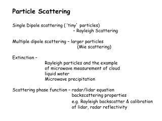
Particle Scattering Single Dipole scattering ( ‘ tiny ’ particles) – Rayleigh Scattering Multiple dipole scattering – larger particles (Mie scattering) Extinction –

E N D
Particle Scattering Single Dipole scattering (‘tiny’ particles) – Rayleigh Scattering Multiple dipole scattering – larger particles (Mie scattering) Extinction – Rayleigh particles and the example of microwave measurement of cloud liquid water Microwave precipitation Scattering phase function – radar/lidar equation backscattering properties e.g.Rayleigh backscatter & calibration of lidar, radar reflectivity
Analogy between slab and particle scattering Insert 13.10/ 14.1 slab particle Slab properties are governed by oscillations (of dipoles) that coherently interfere with one another creating scattered radiation in only two distinct directions - particles scatter radiation in the same way but the interference are less coherent producing scattered stream of uneven magnitude in all directions
Radiation from a single dipole* Scattered wave is spherical in wave form (but amplitude not even in all directions) Scattered wave is proportional to the local dipole moment (p=E) Basic concept of polarization • Key points to note: • parallel & perpendicular • polarizations • scattering angle Any polarization state can be represented by two linearly polarized fields superimposed in an orthogonal manner on one another * Referred to as Rayleigh scattering
Scattering Regimes From Petty (2004)
Rayleigh Scattering Basics Single-particle behavior only governed by size parameter and index of refraction m!
Rayleigh “Phase Function” Vertical Incoming Polarization Horizontal Incoming Polarization Incident Light Unpolarized
Polarization by Scattering Fractional polarization for Rayleigh Scattering The degree of polarization is affected by multiple scattering. Position of neutral points contain information about the nature of the multiple scattering and in principle the aerosol content of the atmosphere (since the Rayleigh component can be predicted with models).
0.04 0 Rayleigh scattering as observed POLDER: Radiance Strong spatial variability Scattering angle Pol. Rad 650 nm Smooth pattern Signal governed by scattering angle (Deuz₫ et al., 1993, Herman et al., 1997) Proportional to Q
Radiation from a multiple dipole particle r ignore dipole-dipole interactions rcos At P, the scattered field is composed on an EM field from both particles size parameter P For those conditions for which =0, fields reinforce each other such that I4E2
Scattering in the forward corresponds to =0 – always constructively add Larger the particle (more dipoles and the larger is 2r/ ), the larger is the forward scattering The more larger is 2r/, the more convoluted (greater # of max-min) is the scattering pattern
Phase Function of water spheres (Mie theory) High Asymmetry Parameter Properties of the phase function asymmetry parameter g=1 pure forward scatter g=0 isotropic or symmetric (e.g Rayleigh) g=-1 pure backscatter • forward scattering & increase with x • rainbow and glory • Smoothing of scattering function by polydispersion Low Asymmetry Parameter
Particle Extinction Particle scattering is defined in terms of cross-sectional areas & efficiency factors σext = effective area projected by the particle that determines extinction Similarly σsca, σabs Geometric cross-section r2 The efficiency factor then follows
Particle Extinction (single particle) =1 Note how the spectrum exhibits both coarse and fine oscillations Implications of these for color of scattered light How Qext2 as 2r/ extinction paradox ‘Rayleigh’ limit x0 (x<<1)
Extinction Paradox shadow area r2 combines the effects of absorption and any reflections (scattering) off the sphere.
insert 14.10 Poisson spot – occupies a unique place in science – by mathematically demonstrating the non-sensical existence of such a spot, Poisson hoped to disprove the wave theory of light.
Mie Theory Equations • Exact Qs, Qa for spheres of some x, m. • a, b coefficients are called “Mie Scattering coefficients”, functions of x & m. Easy to program up. • “bhmie” is a standard code to calculate Q-values in Mie theory. • Need to keep approximately x + 4x1/3 + 2 terms for convergence
Volumes containing clouds of many particles Extinctions, absorptions and scatterings by all particles simply add- volume coefficents half of 14.9 L-4 L L-1 L2 n( r)= the particle size distribution # particles per unit volume per unit size r Exponential distribution (rain) Modified Gamma distribution (clouds) Lognormal distribution (aerosols, sometimes clouds)
Effective Radius & Variance Mean particle radius – doesn’t have much physical relevance for radiative effects For large range of particle sizes, light scattering goes like πr2. Defines an “effective radius” “Effective variance” Modified Gamma distribution a = effective radius b = effective variance
Polydisperse Cloud: Optical Depth, Effective Radius, and Water Path (visible/nir ’s) Cloud Optical Depth Volume Extinction Coefficient [km-1] Cloud Optical Depth Local Cloud Density [kg/m3] Cloud Effective Radius [μm] 1st indirect aerosol effect! (Twomey Effect) ρcloudz
Variations of SSA with wavelength Somewhat Absorbing Non-Absorbing!
Satellite retrieve of cloud optical depth & effective radius Absorbing Wavelength (<1): Reflectivity is mainly a function of cloud droplet size (for thicker clouds). Non-absorbing Wavelength (~1): Reflectivity is mainly a function of optical depth.
The reflection function of a nonabsorbing band (e.g., 0.66 µm) is primarily a function of cloud optical thickness • The reflection function of a near-infrared absorbing band (e.g., 2.13 µm) is primarily a function of effective radius • clouds with small drops (or ice crystals) reflect more than those with large particles • For optically thick clouds, there is a near orthogonality in the retrieval of tc and re using a visible and near-infrared band • re usually assumed constant in the vertical. Therefore:
Cloud Optical Thickness and Effective Radius(M. D. King, S. Platnick – NASA GSFC) Cloud Optical Thickness Cloud Effective Radius (µm) 1 10 >75 1 10 >75 6 17 28 39 50 2 9 16 23 30 Ice Clouds Water Clouds Ice Clouds Water Clouds King et al. (2003)
Monthly Mean Cloud Effective RadiusTerra, July 2006 • Liquid water clouds • Larger droplets in SH than NH • Larger droplets over ocean than land (less condensation nuclei) • Ice clouds • Larger in tropics than high latitudes • Small ice crystals at top of deep convection
Aerosol retrieval from space- the MODIS aerosol algorithm • Uses bi-modal, log-normal aerosol size distributions. • 5 small - accumulation mode (.04-.5 m) • 6 large - coarse mode (> .5 m) • Look up table (LUT) approach • 15 view angles (1.5-88 degrees by 6) • 15 azimuth angles (0-180 degrees by 12) • 7 solar zenith angles • 5 aerosol optical depths (0, 0.2, 0.5, 1, 2) • 7 modis spectral bands (in SW) • Ocean retrievals • compute IS and IL from LUT • find ratio of small to large modes () and • the aerosol model by minimizing and Im is the measured radiance. • then compute optical depth from • aerosol model and mode ratio.
Land retrievals • Select dark pixels in near IR, • assume it applies to red and blue • bands. • Using the continental aerosol model, • derive optical depth & aerosol models (fine & course modes) that best fit obs (LUT approach including multiple scattering). • The key to both ocean and land retrievals is that the surface reflection is small.
“Deep Blue” MODIS Algorithm works over Bright Surfaces • Uses fact that bright surfaces are often darker in blue wavelengths • Uses 412 nm, 470nm, and 675nm to retrieve AOD over bright surfaces. • Still a product in its infancy
“Deep Blue” MODIS Algorithm works over Bright Surfaces • Uses fact that bright surfaces are often darker in blue wavelengths • Uses 412 nm, 470nm, and 675nm to retrieve AOD over bright surfaces. • Complements “Dark Target” retrieval well. • Still being improved!
spheres spherical Non spherical with plane of symmetry non spheres
Particle Backscatter Cd()I0 is the power scattered into per unit solid angle Differential cross-section Bi-static cross-section Backscattering cross-section CbI0 is the total power assuming a particle scatters isotropically by the amount is scatters at =180
Polarimetric Backscatter: LIDAR depolarization • Transmit linear • Receive parallel/perpendicular Ice Water/Ice/Mix =0 for spheres
Polarimetric Backscatter: RADAR ZDR • Transmit both horizontal & vertical • Receive horizontal & vertical for spheres, ZDR~0
Lidar Calibration using Rayleigh scattering Laser backscattering Crossection as measured During the LITE experiment For Rayleigh scattering
Lidar Calibration using Rayleigh scattering Rayleigh scattering is well-understood and easily calculable anywhere in the atmosphere! ns= 1 + a * (1 + b λ-2) Stephens et al. (2001)