Understanding Random Numbers and Probability Distributions
340 likes | 442 Vues
Learn about probability distributions, expectation values, variances, Chebyshev's inequality, and generating random numbers. Explore different distributions and their applications in statistics.

Understanding Random Numbers and Probability Distributions
E N D
Presentation Transcript
4.1.2.2.2 Random Numbers and Distributions Session 2 • probability distributions 2.1.2.4.2 - Random Numbers and Distributions
last time • computers cannot generate real random numbers, only pseudo-random numbers • PRNs are drawn from a deterministic sequence, with possibly a very large period • Marsenne Twister has a period of ~220,000 • linear congruential generators (LCG) are a very common method of generating PRNs • modified LCGs are at the heart of many PRNGs like ANSI C rand(), drand48() and others • LCG values do not fill space evenly • choose a,c,m carefully • do not choose a,c,m yourself • random.mat.sbg.ac.at/~charly/server/node3.html • LCG sequences can fail randomness tests well before the end of their period • Park-Miller minimal standard fails chi-squared after 107 numbers (<1% of its period) 2.1.2.4.2 - Random Numbers and Distributions
probability distributions • the statistical outcome of random processes can frequently be described by using a probability distribution • if the observed outcomes are , then the probability distribution gives the chance of observing any one of the outcomes. • for a fair coin, there are two outcomes, heads (H) or tails (T) • these are examples of a finite random variable – number of outcomes are finite 2.1.2.4.2 - Random Numbers and Distributions
graphing probability distributions • probability distributions are drawn as column graphs when the number of outcomes is small single toss of a fair coin two tosses of a fair coin P=1/2 P=1/4 P=1/4 outcome number of heads in 2 tosses 2.1.2.4.2 - Random Numbers and Distributions
expectation value • the average or expectation value of a random variable is given in terms of the probability distribution • E(x) is a weighted average, with the weights of each outcome being the probability of that outcome • for two tosses of a coin, the average number of heads in two tosses is number of heads, nh probability of observing nh heads 2.1.2.4.2 - Random Numbers and Distributions
expectation value • if the random variable is uniformly distributed, then P(x) is constant • if there are n outcomes, the requirement implies • the expectation value reduces to the familiar form of the average • commonly is used to indicate the expectation value 2.1.2.4.2 - Random Numbers and Distributions
variance • the variance gives a sense of the dispersion of the random values away from the expectation value • the variance is given by • this looks just like an expectation value – and it is, but not of the variable but of a transform of the variable – the square of the distance from the average • the standard deviation, , is related to the variance 2.1.2.4.2 - Random Numbers and Distributions
standardized random variable • the overall shape of the probability distribution function is of most importance • for different values of the mean, the distribution will be “centered” at a different value • for different values of the variance, the distribution will be “stretched” differently • mean and variance are parameters, not fundamental descriptors of the distribution • standardized random variable is a transformation • Z is used to describe the underlying nature of a process (e.g. cars arriving at a traffic light), whereas X describes a particular instance (e.g. cars arriving at a traffic light in rush hour) 2.1.2.4.2 - Random Numbers and Distributions
chebyshev’s inequality • the variance measures the spread of values about the mean • the smaller the variance, the more tightly values are grouped around the mean • Chebyshev’s inequality puts a lower bound on the probability of finding a random variable within a multiple of the standard deviation • recall that for a normal distribution, a value will land within 68% of the time (2 95%) • for any random variable, • probability of falling within 2 is at least 75% • ... within 3 is at least 89% • ... within 4 is at least 94% 2.1.2.4.2 - Random Numbers and Distributions
cumulative probability distribution • the probability distribution P(x) gives you the chance of observing an event, x • the cumulative distribution F(x) gives you the chance of observing any event x probability of observing exactly nh heads probability of observing nh or fewer heads number of heads, nh, in 2 tosses 2.1.2.4.2 - Random Numbers and Distributions
generating numbers from arbitrary distributions • let’s use the coin example to generate random numbers from a non-uniform distribution • the distribution will correspond to the number of heads in two tosses of a coin • generate 0 25% of the time • generate 1 50% of the time • generate 2 25% of the time • we can use the cumulative distribution and a uniform random number generator • each URD will be mapped onto an outcome that is distributed according to our probability distribution 2.1.2.4.2 - Random Numbers and Distributions
using cumulative distribution to generate random values URD [0,1) 0.68 0.68 maps onto 1 2.1.2.4.2 - Random Numbers and Distributions
using cumulative distribution to generate random values # generate a uniform random deviate my $urd = rand(); # define the cumulative distribution function # c(0) = 0.25, c(1) = 0.75, c(2) = 1 my @c = (0.25,0,75,1); # find the smallest i for which urd <= c(i) for my $i (0..@c-1) { return $i if $urd <= $c[$i]; } 25% of URDs fall here 50% of URDs fall here 25% of URDs fall here 2.1.2.4.2 - Random Numbers and Distributions
rejection method 2.1.2.4.2 - Random Numbers and Distributions
continuous random variables • not all random variables are finite • toss of a coin or die is finite • heights of individuals is not finite • height can be any real number in a practical range, e.g. 0 – 3 meters • number of different heights in this range is infinite • the probability and cumulative distribution functions are replaced by continuous equivalents • sums are now integrals 2.1.2.4.2 - Random Numbers and Distributions
uniform distribution • the uniform distribution is the distribution from which PRNGs sample their values P(x) F(x) 2.1.2.4.2 - Random Numbers and Distributions
distributions • bernoulli • geometric • binomial • normal • poisson • exponential 2.1.2.4.2 - Random Numbers and Distributions
bernoulli distribution • an experiment in which there can be only two outcomes is a Bernoulli trial • typically labeled as success (value 1) or failure (value 0) • probability of success is p • probability of failure is 1-p=q • E(X)=p var(X)=p(1-p) • to generate a Bernoulli variable, compare an URD to the success probability • return 1 if URD is smaller than success • return 0 otherwise my $brd1 = rand() < $p; # or equivalently my $brd2 = rand() > $q; 2.1.2.4.2 - Random Numbers and Distributions
geometric distribution • given a Bernoulli trial with probability of success p, the geometric distribution describes the probability of obtaining a success (S) after exactly n failures (F) • n=0 : S • n=1 : FS • n=2 : FFS • n=3 : FFFS, etc • P(X=n)=(1-p)np E(X) = 1/p P(Xn)=1-qn+1 • given a die, the probability or tossing a “1” is 1/6 • the probability of having to toss the die 9 times before seeing a 1 (on the 10th toss) is 2.1.2.4.2 - Random Numbers and Distributions
generating geometric distribution • transforming a uniform distribution to geometric distribution can be done via the cumulative form of the geometric distribution cumulative distribution URD [0,1) probability distribution 2.1.2.4.2 - Random Numbers and Distributions
generating geometric distribution • I generated 10,000 values from the geometric distribution with p=q=0.5 # generate a uniform random deviate my $urd = rand(); # walk along cumulative distribution until # the URD is smaller my $i = 0; while( $urd > 1-$q**($i+1)) { $i++; } print $urd,$i; 2.1.2.4.2 - Random Numbers and Distributions
binomial distribution • the geometric distribution gives the probability of success after n failures, but... • the binomial distribution gives the probability of k success after n trials in a Bernoulli process with success probability p probability of obtaining n-k failures probability of obtaining k successes number of ways k successes can appear in n trials 2.1.2.4.2 - Random Numbers and Distributions
binomial distribution • consider k=2 and n=3 and p=0.5 • seek the probability of 2 successes out of 3 trials • there are three ways in which this can happen • SSF • SFS • FSS • the binomial coefficient for C(3,2)=3 multiples the probability pkqn-k to correct for the fact that the outcome may manifest itself in more than one way • E(X) = np var(X) = npq • consider a box of 12 lighbulbs - if the chance that any one bulb is broken is 0.01 • 89% of the time there will be no broken bulbs, P(n=12,k=0,p=0.01) • 99.4% of the time there will be no more than one broken bulb, P(12,0,0.01)+P(12,1,0.01) • 99.98% of the time there will be no more than two broken bulbs 2.1.2.4.2 - Random Numbers and Distributions
normal distribution • the binomial distribution approaches the normal distribution when • n is very large • p is fixed • regime for np,nq>5 and • plot at right shows normal and binomial distributions for n=6 and p=0.5 2.1.2.4.2 - Random Numbers and Distributions
normal distribution 2.1.2.4.2 - Random Numbers and Distributions
normal distribution • the normal distribution is extremely common in physical and psychological sciences • underlying causes of phenomena are unknown, but small effects are added into an observable score • central limit theorem popularizes the normal distribution • take a collection of random values from the same distribution which has a given mean and standard deviation • compute the average of these values • if you repeat this experiment, the average will be normally distributed 2.1.2.4.2 - Random Numbers and Distributions
poisson distribution • the binomial distribution is approximated by the poisson distribution when • n is very large • p is very small • = np • Poisson distribution describes the number of events in unit time, if the events occur at a fixed rate • consider cars arriving at a traffic light at the rate of 1 per minute. In a 10 minute period, you expect 10 cars (this is the average and the value of above) • what is the probability that you’ll see only 5 cars in this time period (10 minutes)? 2.1.2.4.2 - Random Numbers and Distributions
poisson distribution • if is taken to be a rate, per unit time, then Poisson gives the probability of a given number of occurrences before time t • in the example before, the rate was =1 car per minute and the probability to calculate was waiting t=10 minutes and seeing only 5 cars • many other occurrences of Poisson exist • number of dead squirrels per unit distance of highway • number of spelling mistakes on a page • number of hits to a web server per minute • number of randomly selected points in a volume of space 2.1.2.4.2 - Random Numbers and Distributions
exponential distribution • this is a continuous version of the geometric distribution we’ve already seen • geometric distribution gave the probability of seeing a success after n failures of a Bernoulli trial • exponential distribution gives the probability of having to wait a given amount of time before an event happens • before your next phone call • before your next email arrives • before your next car accident 2.1.2.4.2 - Random Numbers and Distributions
waiting for him/her to call • suppose your boy/girl-friend calls you at a rate of once per 12 hour period (=1/12), what is the probability that you’ll have to wait more than 24 hours before their call? • the event (phone call) happens at a rate of =1/12 • Poisson would tell us how many calls we can expect in a given time • e.g. probability of receiving 2 calls in 1 hour, 2 calls in 2 hours, 3 calls in 10 hours etc • exponential distribution tells us how long we need to wait before the next event (inter-event time) number of events (poisson) t waiting time (exponential) 2.1.2.4.2 - Random Numbers and Distributions
waiting for him/her to call • the cumulative form of the exponential distribution gives us the probability that the waiting time is less than a certain value • p = probability of waiting more than 24 hours • 1 – p = probability of waiting less than 24 hours • thus the probability of waiting more than 24 hours without a call is 0.14. 2.1.2.4.2 - Random Numbers and Distributions
Math::CDF • this module gives both probability and cumulative distributions • cumulative probability PXXXX • quantile probability QXXXX pbeta(), qbeta() [Beta Distribution] pchisq(), qchisq() [Chi-square Distribution] pf(), qf() [F Distribution] pgamma(), qgamma() [Gamma Distribution] pnorm(), qnorm() [Standard Normal Dist] ppois(), qpois() [Poisson Distribution] pt(), qt() [T-distribution] pbinom() [Binomial Distribution] pnbinom() [Negative Binomial Distribution] # -1.96 – value at which probability is 0.025 that (X-)/ (X normally distributed) is smaller qnorm(0.025) 2.1.2.4.2 - Random Numbers and Distributions
Math::Random • provides random values sampled from variety of distributions random_beta random_chi_square random_exponential random_f random_gamma random_multivariate_normal random_multinomial random_noncentral_chi_square random_noncentral_f random_normal random_permutation random_permuted_index random_uniform random_poisson random_uniform_integer random_negative_binomial random_binomial random_seed_from_phrase random_get_seed random_set_seed_from_phrase random_set_seed # generate 100 normally distributed random numbers # with average 10 and stdev 0.5 random_normal(100, 10, 0.5) 2.1.2.4.2 - Random Numbers and Distributions
4.1.2.2.2 Random Numbers and Distributions Session 2 • lots of distributions exist • search for “random” on CPAN 2.1.2.4.2 - Random Numbers and Distributions