Download
1 / 28
280 likes | 402 Vues
This guide provides step-by-step instructions on how to export data from Aware to an Excel spreadsheet and reformat cells containing green triangles to ensure proper data manipulation. Learn to highlight and apply conditional formatting in Excel, including filling in cells based on specific conditions. Create rules for highlighting data within defined ranges and manage existing formatting rules effectively. Additionally, discover how to convert percentage values properly and save your document using the appropriate settings.

E N D
Exporting Data in Aware to an Excel Spreadsheet
All data cells that contain a green triangle need to be reformatted by Excel in order for the data to be manipulated correctly. After the data is highlighted a yield sign will appear in the corner of the highlighted data.
The data now must be reformatted by Excel to accept changes. This data must be converted to a Number.
After selecting the data, choose the Conditional Formatting button on the ribbon and follow the highlighted selections in the drop down menus.
Choose Format only cells that contain and then fill in the rule description with the appropriate numbers that fit your range of data.
Create the cell formatting by clicking on the Format tab. Notice that the Preview shows no current formatting selected.
Select the Fill tab and then choose the color of your choice. The Sample will fill to the color you selected. Choose Clear to change to another color, OK to use the selected color, or Cancel to move back in the process.
The formatting shows up in the column which was selected earlier. These cells contain data found within the range of the first rule.
To create a second rule go back through the same procedure as describe in Slide # 9 of this instructional PowerPoint.
A second rule has been created with Green highlighting all scores that fall between 16 and 18 in the column.
The formatting shows up in the column which was selected earlier showing red for the first rule and green for the second rule.
To edit the rules you can move to the Manage rules menu and edit the rules that appear for this document.
Now all three rules appear in the Rules Manager and are available for editing.
Data cells containing numbers with percents are treated a bit differently. Notice the green triangle? That column needs to be converted to a number. Highlight the cell, click the yield sign and select Convert to a Number If you select a column to format that contains a percentage, the rule values must contain the percent sign.
If you select a column to format that contains a percentage, the rule values must contain the percent sign.
To save the document, click on the Office button, choose Save as… and then Save a copy of the document which works best for you.