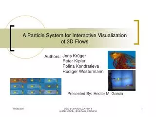
Interactive Terascale Particle Visualization
Interactive Terascale Particle Visualization. Ellsworth, Green, Moran (NASA Ames Research Center). Motivation. Produce an interactive visualization of a 2TB CFD data set using particle tracing. Precomputation of a large number of particles on a PC cluster Out-of-core interactive visualization.

Interactive Terascale Particle Visualization
E N D
Presentation Transcript
Interactive Terascale Particle Visualization Ellsworth, Green, Moran (NASA Ames Research Center)
Motivation • Produce an interactive visualization of a 2TB CFD data set using particle tracing. • Precomputation of a large number of particles on a PC cluster • Out-of-core interactive visualization
Overview • Computing streaklines and storing them on disk for a visualization application to retrieve data as needed. • Computed streakline data contains position and several scalar values like particle age, pressure, etc.
Algorithm Overview • Computes particle traces and scalar values • One file per timestep, streaklines are stored contiguously (single disk read). • Variable-length traces are stored according to Morton (space filling curve) order for locality. • Coordinates are downsampled to 16bit, so are scalar values at each position. • Scalar values are stored in separate files.
Curvilinear Grid • Seedpoints on a regulargrid might fall outside the curvilinear grid (86 % outside in this case. • Thus, check seedpoint in every timestep and mark active seedpoints (active in all timesteps)
Particle Computation • done on a 49-node Beowolf cluster. • Streakline computation is independent, but input data is too big (2 TB). • Each node gets chunks of seedpoints to compute. • What can be done about reducing the memory footprint?
Exploiting Mesh Regularities • Some zones of the mesh do not change over time, others are rotated copies of other zones, etc. • Automatically find regularities and replace mesh with a new version. • Replacement mesh cuts down the amount of data by a factor of over 5000.
Demand-Paging Data • As only parts of the domain are needed, it is divided up into a number of fixed-size blocks. • Then use demand-paging algorithm (with LRU replacement) to keep memory footprint reasonable. • Use several threads per node to keep CPU utilization high. • Prefetch data for newly loaded timestep.
Computation Performance • Fairly slow: 5 days for the 2 TB dataset, producing 1.7 GB of uncompressed particle data (293 billion particles) • Threading library seems to have a huge impact on performance…
Particle Trace Compression • Use previous values in sequence to predict future values (0th, 1st, 2nd order prediction) and compress using zlib.
Viewer Program • Client with file server architecture • Viewer allows viewpoint manipulation and seedpoint selection (using an axis-aligned selection box) • Very similar to our “dmqr” in terms of server/client communication for queries.
Results • Equipment used includes: • 49-node Beowolf cluster, 1.7GHz Athlon MP, 1GB memory, Fast Ethernet. • Master node: 1.7GHz Athlon MP, 2GB memory, Gigabit Ethernet. • File servers: 3GHz Dual Xeon, 4GB memory, Gigabit Ethernet, 21250GB storage (RAID 5 => 4.5 TB total storage available) • Viewer ran on: 3GHz Dual Xeon, 4GB memory, Gigabit Ethernet, NVIDIA Quattro FX