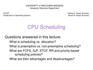
CPU Scheduling
CPU Scheduling. ICS 240: Operating Systems William Albritton Information and Computer Sciences Department at Leeward Community College Original slides by Silberschatz, Galvin, and Gagne from Operating System Concepts with Java, 7th Edition with some modifications

CPU Scheduling
E N D
Presentation Transcript
CPU Scheduling ICS 240: Operating Systems William Albritton Information and Computer Sciences Department at Leeward Community College Original slides by Silberschatz, Galvin, and Gagne from Operating System Concepts with Java, 7th Edition with some modifications Also includes material by Dr. Susan Vrbsky from the Computer Science Department at the University of Alabama 6/6/2014 1
Class Feedback • On an anonymous (don’t write your name) sheet of paper, answer the following questions • Average time working on each assignment • Total time studying for the exam • List several things that help you learn • List several things that make learning difficult • List several suggestions for improving the class
Basic Concepts • Maximum CPU utilization obtained with multiprogramming • CPU–I/O Burst Cycle • Process execution consists of a cycle of CPU execution and I/O wait • CPU burst: a time interval when a process uses the CPU only (few long CPU bursts) • I/O burst: a time interval when a process uses I/O devices only (more short CPU bursts) • CPU burst distribution (next two slides)
Histogram of CPU-burst Times • This histogram (a graphical display of a frequency distribution) shows many, short CPU bursts and a few, long CPU bursts.
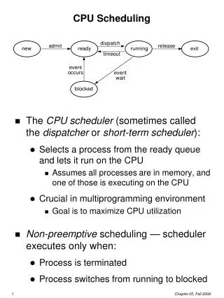
CPU Scheduler • Short-term scheduler • Selects from among the processes in memory (in the ready queue) that are ready to execute, and allocates the CPU to one of them • Note that the ready queue is not necessarily a first-in first-out (FIFO) queue, as different algorithms other than first-in first-out (FIFO) might be used to manage the queue • For example, a queue at a club is not necessarily first-in first-out (FIFO), as VIPs usually jump to the front of the queue • A queue is a fancy word for line
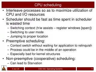
Preemptive vs. Non-preemptive Non-preemptive scheduling scheme The short-term scheduler cannot forcibly take the CPU back from a process Once the CPU has been allocated to a process, the process keeps the CUP until the process releases the CPU either by terminating or by switching to the waiting state Also called cooperative scheduling scheme
Preemptive vs. Non-preemptive Preemptive scheduling scheme The short-term scheduler takes the CPU from the process Can take the CPU back due to Time slice Higher priority process arrived Interrupts
Process State • As a process executes, it changes state • new: The process is being created • running: Instructions are being executed • waiting: The process is waiting for some event to occur • For example, I/O completion or reception of a signal • ready: The process is waiting to be assigned to a processor • terminated: The process has finished execution
CPU Scheduler CPU scheduling decisions (by the short-term scheduler) may take place when a process Switches from running to waiting state For example, when the process has an IO request This is non-preemptive Switches from running to ready state For example, when an interrupt occurs This is preemptive
CPU Scheduler CPU scheduling decisions (by the short-term scheduler) may take place when a process Switches from waiting to ready state For example, at the completion of I/O This is preemptive Terminates For example, the process (running program) is done This is non-preemptive
Dispatcher • Dispatcher module gives control of the CPU to the process selected by the short-term scheduler • This function involves the following steps • switching context • switching to user mode • jumping to the proper location in the user program to restart that program
Dispatcher • Because the dispatcher is used during every process switch, the dispatcher should be as fast as possible • Dispatch latency • time it takes for the dispatcher to stop one process and start another running
Scheduling Criteria • The following 5 factors are used as Scheduling Criteria (Performance Evaluation), which are used to compare CPU scheduling algorithms • CPU utilization • Fraction of time CPU busy (through multiprogramming) • Range from 40% (light load) to 90% (heavily used) • goal: maximize • Throughput • Number of processes that complete their execution per time unit (measure of work) • Range from one process per hour to ten processes per second • goal: maximize
Scheduling Criteria • The following 5 factors are used as Scheduling Criteria (Performance Evaluation), which are used to compare CPU scheduling algorithms • Turnaround time • Amount of time to execute a particular process • In other word, the delay between job submission and job completion • The sum of the time waiting to get into memory, waiting in the ready queue, executing on the CPU, and doing I/O • goal: minimize
Scheduling Criteria The following 5 factors are used as Scheduling Criteria (Performance Evaluation), which are used to compare CPU scheduling algorithms Waiting time Amount of time a process has been waiting in the ready queue Note that a CPU scheduling algorithm cannot change the execution time or I/O goal: minimize Response time Amount of time it takes from when a request was submitted until the first response is produced In other words, the amount of time from request until the process starts to respond goal: minimize
Optimization Criteria • Max CPU utilization • Max throughput • Min turnaround time • Min waiting time • Min response time
FCFS Scheduling FCFS - First Come First Serve The process that requests the CPU first is allocated to the CPU first Simple and non-preemptive Better to schedule shorter processes before longer ones Convoy effect happens when short process get stuck behind long process Unfair to processes with short bursts Not usually used alone, but as a part of a more complex algorithm
P1 P2 P3 0 24 27 30 FCFS Scheduling ProcessBurst Time P1 24 P2 3 P3 3 • Suppose that the processes arrive in the order: P1 , P2 , P3 all at time 0. The Gantt Chart for the schedule is: • Throughput: 3 processes/30 milliseconds = 1/10 • Turnaround time for P1 = 24; P2 = 27; P3 = 30 • Average turnaround time: (24 + 27 + 30)/3 = 81/3 = 27 • Waiting time for P1 = 0; P2 = 24; P3 = 27 • Average waiting time: (0 + 24 + 27)/3 = 51/3 = 17
P2 P3 P1 0 3 6 30 FCFS Scheduling Suppose that the processes arrive in the order P2 , P3 , P1 all at time 0 • The Gantt chart for the schedule is: • Throughput: 3 processes/30 milliseconds = 1/10 • Turnaround time for P1 = 30; P2 = 3; P3 = 6 • Average turnaround time: (30 + 3 + 6)/3 = 39/3 = 13 • Waiting time for P1 = 6;P2 = 0; P3 = 3 • Average waiting time: (6 + 0 + 3)/3 = 9/3 = 3 • Much better than previous case!
Shortest-Job-First (SJF) Scheduling • Associate with each process the length of its next CPU burst. • Use these lengths to schedule the process with the shortest time first • Non-preemptive • once CPU given to the process it cannot be preempted until completes its CPU burst • SJF is optimal non-preemptive algorithm • Gives minimum average waiting time for a given set of processes
Example of SJF Process Arrival TimeBurst Time P1 0.0 7 P2 0.0 4 P3 0.0 1 P4 0.0 4 • Suppose that the processes arrive in the order: P1 , P2 , P3 , P4 all at time 0. The Gantt Chart for the schedule is | P3 | P2 | P4 | P1 | 0 1 5 9 16 • Throughput: 4 processes/16 milliseconds = 1/4 • Turnaround time for P1 = 16; P2 = 5; P3 = 1; P4 = 9 • Average turnaround time: (16 + 5 + 1 + 9)/4 = 31/4 = 7.75 • Waiting time for P1 = 9;P2 = 1;P3 = 0 ; P4 = 5 • Average waiting time: (9 + 1 + 0 + 5)/4 = 15/4 = 3.75
Process Arrival TimeBurst Time P1 0.0 7 P2 2.0 4 P3 4.0 1 P4 5.0 4 Throughput: 4 processes/16 milliseconds = 1/4 Turnaround time for P1 = 7-0 = 7; P2 = 12-2 = 10; P3 = 8-4 = 4; P4 = 16-5 = 11 Average turnaround time: (7 + 10 + 4 + 11)/4 = 32/4 = 8 Waiting time for P1 = 0-0 = 0;P2 = 8-2 = 6;P3 = 7-4 = 3; P4 = 12-5 = 7 Average waiting time: (0 + 6 + 3 + 7)/4 =16/4 = 4 Another Example of SJF P1 P3 P2 P4 0 3 7 8 12 16
SRTF - Shortest Remaining Time First Preemptive version of Shortest-Job-First (SJF) Scheduling Preemptive If new process arrives with CPU burst less than time left of process currently executing, then new process gets the CPU SRTF is optimal preemptive algorithm Gives minimum average waiting time for a given set of processes 6/6/2014 25
P1 P2 P3 P2 P4 P1 11 16 0 2 4 5 7 Example of SRTF Process Arrival TimeBurst Time P1 0.0 7 P2 2.0 4 P3 4.0 1 P4 5.0 4 • Throughput: 4 processes/16 milliseconds = 1/4 • Turnaround time for P1 = 16-0 = 16; P2 = 7-2 = 5; P3 = 5-4 = 1; P4 = 11-5 = 6 • Average turnaround time: (16 + 5 + 1 + 6)/4 = 28/4 = 7 • Waiting time for P1 = 11-2 = 9;P2 = 5-4 = 1;P3 = 4-4 = 0; P4 = 7-5 = 2 • Average waiting time: (9 + 1 + 0 +2)/4 = 12/4 = 3
Determining Length of Next CPU Burst • For the SJF and SRTF scheduling algorithms, knowing the exact length of the next CPU burst is difficult • For long-term scheduling, the user-defined process time limit can be used • The user has the responsibility for estimating the process time limit accurately • The short-term scheduler does not know the exact length of the next CPU burst • Instead, the next CPU burst is estimated
Determining Length of Next CPU Burst For short-term scheduling, the length of next CPU burst is estimated by using the length of previous CPU bursts, using exponential averaging 6/6/2014 28
Examples of Exponential Averaging • =0 • n+1 = n • Recent history does not count • =1 • n+1 = tn • Only the actual last CPU burst counts • If we expand the formula, we get: n+1 = tn+(1 - ) tn-1+ … +(1 - )j tn-j+ … +(1 - )n +1 0 • Since both and (1 - ) are less than or equal to 1, each successive term has less weight than its predecessor
Priority Scheduling • A priority number (integer) is associated with each process • The CPU is allocated to the process with the highest priority • In this class, assume that the smallest integer has the highest priority • Can be either way, so we will stick with the smallest number for the highest priority to try to avoid confusion • Can be preemptive or non-preemptive
Priority Scheduling Problem of Starvation Low priority processes may never execute Solution is Aging As time progresses, increase the priority of the process By the way, SJF and SRTF are also a type of priority scheduling algorithm Priority is the predicted next CPU burst time 6/6/2014 32
ProcessPriorityBurst Time P1 3 10 P2 1 1 P3 4 2 P4 5 1 P5 2 5 Suppose that the processes arrive in the order: P1 , P2 , P3 , P4 , P5 all at time 0. The Gantt Chart for the schedule is | P2 | P5 | P1 | P3 | P4 | 0 1 6 16 18 19 Throughput: 5 processes/19 milliseconds = 5/19 Turnaround time for P1 = 16; P2 = 1; P3 = 18; P4 = 19; P5 = 6 Average turnaround time: (16 + 1 + 18 + 19 + 6)/4 = 60/5 = 12 Waiting time for P1 = 6;P2 = 0;P3 = 16; P4 = 18; P5 = 1 Average waiting time: (6 + 0 + 16 + 18 + 1)/4 = 41/5 = 8.2 Priority Scheduling (Non-preemptive) 6/6/2014 33
Round Robin (RR) • Each process gets a small unit of CPU time (time quantum or time slice), usually 10-100 milliseconds (ms) • After this time has elapsed, the process is preempted and added to the end of the ready queue • If there are n processes in the ready queue and the time quantum is q • Then each process gets 1/n of the CPU time in chunks of at most q time units at once
P1 P2 P3 P4 P1 P3 P4 P1 P3 P3 0 20 37 57 77 97 117 121 134 154 162 Example of RR ProcessBurst TimeArrival Time P1 53 0 P2 17 0 P3 68 0 P4 24 0 • Time Quantum = 20 ms • Throughput: 4 processes/162 milliseconds = 2/81 • Turnaround time for P1 = 134; P2 = 37; P3 = 162; P4 = 121 • Average turnaround time: (134 + 37 + 162 + 121)/4 = 454/4 = 113.5 • Waiting time for P1 = (77-20)+(121-97) = 81;P2 = (20-0)=20;P3 = (37-0)+(97-57)+(134-117)=94; P4 = (57-0)+(117-77) = 97 • Average waiting time: (81 + 20 + 94 +97)/4 = 292/4 = 73.0
P1 P1 P2 P1 P3 P4 P3 P4 P3 P3 0 20 40 57 70 90 110 130 134 154 162 RR with Different Arrival Times ProcessBurst TimeArrival Time P1 53 0 P2 17 30 P3 68 50 P4 24 60 • Time Quantum = 20 ms • Throughput: 4 processes/162 milliseconds = 2/81 • Turnaround time for P1 = 70-0 = 70; P2 = 57-30 = 27; P3 = 162-50 = 112; P4 = 134-60 = 74 • Average turnaround time: (70 + 27 + 112 + 74)/4 = 283/4 = 70.75 • Waiting time for P1 = (57-40) = 37;P2 = (40-30) = 10;P3 = (162-68-50)=44; P4 = (134-24-60) = 50 • Average waiting time: (37 + 10+ 44 + 50)/4 = 141/4 = 35.25
Time Quantum • How to choose value for time quantum (time slice)? • If time quantum (time slice) is 20 milliseconds and context switch is 5 milliseconds • then 20% wasted on overhead to improve • If time quantum is 500 milliseconds and context switch is 5 milliseconds • then only 4% overhead
Time Quantum • If time quantum (slice) is too small • Overhead of context switch becomes dominant • If time quantum (slice) too large • RR degenerates to FCFS (First Come First Serve) • Typical to have 80% of CPU bursts shorter than time slice • If processes finish CPU burst in single time quantum • The turnaround time will be shorter
Time Quantum & Context Switches • This figure shows how decreasing the time quantum increases the number of context switches
Turnaround Time Varies With The Time Quantum • The average turnaround time does not necessarily improve as the time quantum size increases
Round Robin (RR) • Tradeoffs • RR typically has a higher average turnaround time than SRTF (Shortest Remaining Time First) • However, RR typically has better response time than SRTF • For RR, the implicit assumption is that all processes are equally important • According to Dr. Tanenbaum, RR is the "oldest, simplest, fairest, and most widely used" of the scheduling algorithms
Multilevel Queue Scheduling • For a multilevel queue scheduling algorithm, the ready queue is partitioned into several separate queues • For example, two queues • Interactive/foreground processes at high priorities • Background/batch processes at low priorities • With a multilevel queue scheduling algorithm, each queue has its own scheduling algorithm • Continuing from the above example • foreground – RR (Round Robin) • background – FCFS (First Come First Serve)
Multilevel Queue Scheduling • Scheduling must be done between the queues • Here are some example choices • Use fixed priority scheduling (serve all processes from the foreground, and then from the background) • Possibility of starvation • Use time slicing (each queue gets a certain amount of CPU time which it can schedule amongst its processes) • 80% to foreground in RR • 20% to background in FCFS • A Multilevel Queue is good for time-sharing systems and favors short jobs
Multilevel Queue Scheduling • In this figure, the ready queue is divided into five (5) separate queues
Multilevel Feedback Queue • In a multilevel queue scheduling algorithm, a process is permanently assigned to a specific queue • A multilevel queue scheduling algorithm has low overhead, but is inflexible • In contrast, in a Multilevel Feedback Queue Scheduling Algorithm, a process moves between the various queues • Processes that wait for too long in a particular queue can be moved to another queue • This kind of aging prevent starvation
Multilevel Feedback Queue • Dynamic priorities (priorities change) for each process • Aging, which prevent starvation, can be implemented in this manner • Design decisions • Scheduling algorithm for each queue • Rule for upgrading/degrading process to higher/lower queue • To which queue do new processes go?
Multilevel Feedback Queue • Typical behavior • Higher priority queues have smaller time slices • If a process uses up its time slice, it moves down a priority • If a process blocks before using time slice, it stays at that priority • New processes go to the highest priority
Example of Multilevel Feedback Queue • Three queues • Q0 – RR time quantum 8 milliseconds • Q1 – RR time quantum 16 milliseconds • Q2 – FCFS
Example of Multilevel Feedback Queue • Scheduling • A new job enters queue Q0which is servedFCFS • When it gains CPU, job receives 8 milliseconds. • If it does not finish in 8 milliseconds, job is moved to queue Q1 • At Q1 job is again served FCFS and receives 16 additional milliseconds • If it still does not complete, it is preempted and moved to queue Q2