Download
1 / 82
850 likes | 1.04k Vues
9. Demand-Side Equilibrium: Unemployment or Inflation?. Contents. Meaning of Equilibrium GDP Mechanics of Income Determination Aggregate Demand Curve Demand-Side Equilibrium and Full Employment Coordination of Saving and Investment Changes on the Demand Side: Multiplier Analysis.

E N D
9 Demand-Side Equilibrium: Unemployment or Inflation?
Contents • Meaning of Equilibrium GDP • Mechanics of Income Determination • Aggregate Demand Curve • Demand-Side Equilibrium and Full Employment • Coordination of Saving and Investment • Changes on the Demand Side: Multiplier Analysis
Real World Puzzle: Why does the Market Permit Unemployment? • Market economies coordinate the decisions of millions of buyers and sellers to ensure the correct amount of C goods are produced with most efficient prod means. • Yet market economies stumble with periodic episodes of mass UE and recessions. • Widespread UE is a failure to coordinate economic activity. • If UE were hired, they could buy the goods firms can’t sell; and revenues from these sales would allow firms to hire the UE.
The Meaning of Equilibrium GDP • Recall: total production (GDP) = total income • But total production need not = total spending • If total expenditures > value of output produced • (1) ↓inventory stocks → signals retailers ↑orders → signals manufacturers ↑ production • (2) if high levels of spending continue to deplete inventories → firms ↑prices • If total expenditures < value of output produced • (1) ↑inventory stocks → signals retailers ↓orders → signals manufacturers ↓ production • (2) if low levels of spending continue → firms ↓prices
The Meaning of Equilibrium GDP • Equilibrium on the Demand-side of the Economy • GDP↑ when total expenditures > GDP • GDP↓ when total expenditures < GDP • Equilibrium can only occur when there is just enough spending to absorb current level of prod. Then producers conclude their Q and P decisions were correct. • Equilibrium: total spending = total production • Firms inventories remain at desired levels → no reason to ∆Q or ∆P
The Mechanics of Income Determination • Expenditure Schedule = table showing the relationship between GDP and total spending • Table 1: • C is the Consumption f(x) • I, G, and X-IM are all fixed regardless of the level of GDP • C + I + G + X-IM = total expenditure
C + I + G C + I + G + ( X – I M ) X – IM = –$100 C + I G = $1,300 C I = $900 FIGURE 1.Construction of the Expenditure Schedule C is the C f(x). It is shifted up by the amount of I ($900) and G ($1,300) and shifted down by the amount of X-IM (-$100). Slope of the expenditure schedule = MPC because I, G, and X-IM are assumed to be constant and do not vary with GDP. 6,100 6,000 Real Expenditure 4,800 3,900 5,200 5,600 6,000 6,400 6,800 7,200 Real GDP
The Mechanics of Income Determination • Use Table 2 to understand why $6,000B must be equilibrium level of output. • Any output below $6,000B → total expenditures > GDP → ↓inventories → ↑production • Any output above $6,000B → total expenditures < GDP → ↑inventories → ↓production • Equilibrium only occurs when Y = C + I + G + X-IM or GDP = total expenditure, which happens at $6,000B.
The Mechanics of Income Determination • Use Figure 2 to show why $6,000B must be the equilibrium level of output. • 45 degree line shows all points where output and spending are equal. • These are all points where the economy can possibly be in equilibrium. • Economy is not always on the 45 degree line but it is always on the expenditure schedule. • Equilibrium is shown where 45 degree line intersects the total expenditure schedule.
Output exceeds spending 45° C + I + G + ( X – I M ) E Equilibrium Spending exceeds output FIGURE 2.Income-Expenditure Diagram Left of point E: total expenditure schedule is above the 45 degree line → spending > GDP → ↓inventories and firms ↑prod. Right of point E: total expenditure schedule is below the 45 degree line → spending < GDP → ↑inventories and firms ↓prod. 7,200 6,800 6,400 6,000 Real Expenditure 5,600 5,200 4,800 0 4,800 5,200 5,600 6,000 6,400 6,800 7,200 Real GDP
The Aggregate Demand Curve • The expenditure schedule is drawn for a fixed P level. • Derive AD curve using the expenditure schedule. • Recall P level shifts C f(x) downward • P level (at fixed levels of DI) purchasing power of wealth by lowering the value of money-fixed assets • P level shifts the expenditure schedule downward • ↓ P level shifts the expenditure schedule upward
The Aggregate Demand Curve • How do changes in the P level impact real GDP on the demand-side of the economy? • ↑P level → ↓expenditures → ↓Equil level of GDP • ↓P level → ↑expenditures → ↑Equil level of GDP • We can now draw an AD curve (in Fig 3) where Y0, Y1, and Y2 correspond to the GDP levels depicted in the 45 degree line diagram.
45 C + I + G + ( X – I M ) 2 C + I + G + ( X – I M ) 0 E 0 C + I + G + ( X – I M ) 1 E 1 45 Y Y Y Y Y Y 1 1 0 0 2 2 FIGURE 3.The Effect of the Price Level on Equilibrium AD E2 E1 P1 Price Level Real Expenditure E0 P0 E2 P2 AD Real GDP Real GDP Change in P level Movement along AD curve
The Aggregate Demand Curve • AD has a (-) slope • ↑P level → ↓C via ↓wealth • ↑P level → ↓X-IM • Note: this also shifts the expenditure schedule down and lowers GDP. • Each expenditure schedule describes only one P level. At different P levels, the expenditure schedule is different so equilibrium GDP is different.
Demand-Side Equilibrium and Full Employment • Will economy achieve full employment without inflation? • If the economy always gravitates toward full employment, then gov should leave the economy alone. • We’ve shown that equil GDP is where 45 degree line intersects the exp schedule, but we haven’t determined if that equil level of GDP is at full employment.
Demand-Side Equilibrium and Full Employment • If equil GDP > full employment level of GDP → economy has inflation. • If equil GDP < full employment level of GDP → economy has unemployment.
Potential GDP 45° F C + I + G + ( X – I M ) E B Recessionary gap 45° FIGURE 4.A Recessionary Gap Full emp = $7,000B and equil GDP = $6,000B. Here exp is too low to have full emp. Happens if C, I, G, or X are weak or P level is “too high.” UE occurs because there isn’t enough output demanded to keep entire L force working. Full emp can be reached if exp schedule shifts up to pt F. This could happen without gov intervention if ↓P level. Real Expenditure 6,000 7,000 Real GDP
Potential 45° GDP Inflationary gap E B C + I + G + ( X – I M ) F 45° FIGURE 5.An Inflationary Gap Full emp = $7,000B and equil GDP = $8,000B. Happens if C, I, G, or X are very high or P level is “too low.” Full emp can be reached if exp schedule shifts down to pt F. This could happen without gov intervention if ↑P level. Real Expenditure 7,000 8,000 Real GDP
The Coordination of Saving and Investment • Must full employ level of GDP be an equilibrium? No! • Ignore G and X-IM then we can restate equil GDP: • Y = C + I • Y – C = I • S = I • Reach full employment equil only if S = I. • If S > I → spending is inadequate to support prod at full emp → GDP falls below potential and there is a recessionary gap. • If I > S → spending exceeds potential GDP → production is above full emp level and there is an inflationary gap.
The Coordination of Saving and Investment • S is decided by households and I is decided by corporate executives and home buyers. • Their decisions are not well coordinated. • Not clear the gov can solve the coordination problem of UE.
Changes on the Demand Side: Multiplier Analysis • Multiplier = (∆ in equil GDP) (∆ in spending that caused the ∆ in GDP) • In Table 3, I rises by $200B (from $900B in Table 1), yet equil GDP rises by $800B (not just $200B). Why? • Multiplier > 1 because one person’s spending is another person’s income. Note: multiplier = 4 here. • spending income • A portion of the ↑ in income is spent on C, creating more income, which in turn creates more C, etc.
TABLE 3.Total Expenditure after a $200 Billion Increase in Investment
45 ° E 1 C C + + I0 I1 + + G G + + ( ( X X – – I I M M ) ) $200 billion E 0 FIGURE 6.Illustration of the Multiplier Multiplier = ∆Y/∆I = $800/$200 = 4 Or multiplier = 1/(1-MPC) = 1/(1-0.75) = 4 Real Expenditure 0 6,000 6,800 Real GDP (or Y)
Changes on the Demand Side: Multiplier Analysis • Multiplier = 1 (1 - MPC) • MPC in U.S. has been estimated to be about 0.95, implying that the multiplier is 20. • In fact, the multiplier in U.S. is < 2. • Factors that reduce the size of the multiplier • International trade • Inflation • Income taxation • Financial system
The Multiplier Is a General Concept • ∆I has same multiplier effect as a ∆C, ∆G, or ∆(X - IM). • Consequently, trade links the GDPs of major economies. • GDP in a foreign country its IM, a portion of which are X from U.S. • Growth in U.S. X has a multiplier effect, ↑GDP in U.S. • Booms and recessions tend to be transmitted across national borders.
The Multiplier and the Aggregate Demand Curve • spending shifts AD by an amount given by the oversimplified multiplier formula (1/(1-MPC)). • In Fig 7, I has risen by $200B which shifts AD out by $800B (i.e., 4 (the multiplier) x $200B).
45 ° C + I + G + (X – I M ) 1 E C + I + G + ( X – I M ) 1 0 $200 billion E 0 6,000 6,800 D D 0 1 E E 0 1 D ( I = $1,100) 1 D ( I = $900) 0 6,800 FIGURE 7.Two Views of the Multiplier Real Expenditure 0 Price Level 100 6,000 Real GDP
Contents • Aggregate Supply Curve • Equilibrium of AD and AS • Inflation and the Multiplier • Recessionary and Inflationary Gaps Revisited • Adjusting to a Recessionary Gap or an Inflationary Gap • Stagflation from an Adverse Supply Shock
The Aggregate Supply Curve • Like AD, AS is a curve and not a fixed number. • Qs by firms depends on prices, wages, other input costs, and technology. • AS represents the relationship between P level and GDP supplied, holding all other determinants of Qs fixed. • AS has a (+) slope → ↑P → ↑Qs • Firms are motivated by profit. • Profit per unit = P – AC
S S FIGURE 1. An Aggregate Supply Curve Price Level Real GDP
Why does the Aggregate Supply Curve have a Positive Slope? • Many input prices are fixed for certain periods of time. • Long-term contracts for L or raw materials • Firms choose Qs by comparing selling prices with production costs which depend on input prices. • If ↑selling prices while input costs are fixed → ↑Qs • If ↓selling prices while input costs are fixed → ↓Qs
Shifts of the Aggregate Supply Curve • Costs of production are constant along the AS curve. • costs of production shifts AS curve • Money wage rate • wages account for more than 70% of all prod costs. • ↑wages → ↓profit at any given P of output → ↓Qs • ↑wages → shifts AS inward and ↓wages → shifts AS outward • Prices of other inputs • ↑P of any input → shifts AS inward and ↓P of any input → shifts AS outward
Shifts of the Aggregate Supply Curve • Technology and productivity • Technological breakthrough that ↑L productivity → ↑output per hour of L → ↑profit per unit → ↑Qs • Technological improvements shift AS outward • Available supplies of labor and capital • AS curve shifts out if L force↑; ↑L quality; or ↑K stock because more output can be produced at any given P level.
S (higher wages) 1 S (lower wages) 0 B A S 1 S 0 FIGURE 2.A Shift of the Aggregate Supply Curve 100 Price Level 5,500 6,000 Real GDP
Equilibrium of Aggregate Demand and Supply • Intersection of AD and AS determine the equilibrium level of real GDP and the P level. • Equilibrium (in Fig 3) occurs at a P level = 100 and GDP = $6,000B. • At higher P levels, like 120, Qs > Qd by $800B → ↑inventories → ↓prices and ↓output. • At lower P levels, like 80, Qd > Qs by $800B → ↓inventories → ↑prices and ↑output.
S D E D S FIGURE 3.Equilibrium Real GDP and the Price Level 130 120 Price Level 110 100 90 80 5,200 5,600 6,000 6,400 6,800 Real GDP
Inflation and the Multiplier • Recall: multiplier effect suggests A’s spending becomes B’s income, and B’s spending becomes C’s income, etc. • Earlier discussion focused on spending and assumed the P level was fixed. • Focused on the D-side equilibrium and ignored the reactions of firms (i.e., the S-side). • Will firms supply the additional demand without ↑P? • Not if AS slopes upward! • Inflation size of the multiplier
Inflation and the Multiplier • In Fig 4, ↑I by $200B which shifts AD out by $800B ($200B x oversimplified multiplier of 4). • Shown by the movement from E0 to A. • Firms react to higher levels of spending (shift of AD at P level = 100) by ↑output and ↑prices. • Shown by the movement from E0 to E1 –along AS curve. • ↑P level → ↓purchasing power of money-fixed assets → ↓C and ↓X-IM • Shown by the movement from A to E1 –along new AD curve. • Multiplier is only 2 now = ∆Y/∆I = $400B/ $200B.
D1 S D0 $800 E1 billion E0 D1 S D0 FIGURE 4.Inflation and the Multiplier Assume I rises by $200B. This raises total expenditure (or Q of AD) by $800 (= $200B x multiplier of 4). If AS were horizontal → multiplier = 4 and equil GDP would rise to $6,800B. If AS were vertical → multiplier = 0 and equil GDP would remain at $6,000B. Here AS is upward sloping and ↑P level with the shift in AD. The multiplier is 2 (= $400B/$200B). 130 120 110 Price Level (Y) 100 90 80 6,000 6,400 6,800 Real GDP (Y) NOTE: Amounts are in billions of dollars per year.
Recessionary and Inflationary Gaps Revisited • Short run: equilibrium of AS and AD may or may not equal full employment GDP • Recessionary gap: equilibrium GDP < full employment or potential GDP • Inflationary gap: equilibrium GDP > full employment or potential GDP • Long run: wages adjust to labor market conditions to make equilibrium GDP = full employment or potential GDP • But this may take a long time!
Adjusting to a Recessionary Gap • In Fig. 5, equil GDP falls below the full employment level. • This might be caused by weak C or low I. • Loose L market • There is UE and jobs are hard to find. • Employees may be anxious to keep their jobs. • Workers won’t win ↑wage and wages might fall. • If ↓wages → AS shifts outward →↓P level and ↓UE • Deflation erodes the recessionary gap –but this process happens very slowly!
Potential GDP S 0 S 1 D E B Recessionary F gap S D 0 S 1 FIGURE 5. The Elimination of a Recessionary Gap Recessionary gap = $1,000B. Weak spending and UE at pt E. Weak labor markets put pressure on wages to fall. Falling wages shift AS outward which lowers prices. Falling prices stimulate C and net X. Price Level 100 6,000 7,000 Real GDP
Adjusting to a Recessionary Gap • In the real economy, however, wage reductions are slow and uncertain, particularly in the post-WWII period. • E.g., even with the severe recession of 1981-82 where UE reached 10%, prices and wages were not forced down –though their rates of increase were.
Adjusting to a Recessionary Gap • Why haven’t wages fallen much since WWII? • Institutional factors: like min wages, union contracts, and gov regulations that place legal floors on wages and prices. These were all developed since WWII. • Psychological resistance: firms are reluctant to cut wages for fear their employees will resent it and reduce effort. • But why wasn’t this true prior to WWII?
Adjusting to a Recessionary Gap • Business cycles were less severe: after WWII so firms and workers wait out the bad times rather than accept wage or price cuts. • Firms lose their best workers: if a firm cuts wages, it may lose its best employees. Individual productivity is hard to measure. The best workers have the greatest opportunities elsewhere. • Should have been true before WWII. • With sticky wages and prices, cyclical unemployment may last a long time.
Adjusting to a Recessionary Gap • Does the Economy Have a Self-Correcting Mechanism? • The economy will self-adjust eventually. • wages demand for labor • prices demand for goods and services • But many people believe that gov intervention should help to speed up the process. • Eg., Recovery from 1990-91 recession took almost 4 years. • UE fell from 7.7% to 5.4% • Inflation fell from 6.1% to 2.7%
Adjusting to a Recessionary Gap • An Example from Recent History: Disinflation in Japan in the 1990s. • Recovery from the 1990-91 recession was weak and long delayed, but it did eventually come. • Practical question: How long can we afford to wait?