Download
1 / 117
1.19k likes | 1.51k Vues
Macroeconomics of Business Cycles. macro . Growth rates of real GDP, consumption. Real GDP growth rate. Consumption growth rate. Average growth rate. Percent change from 4 quarters earlier. Growth rates of real GDP, consumption, investment. Real GDP growth rate. Investment growth rate.

E N D
Growth rates of real GDP, consumption Real GDP growth rate Consumption growth rate Average growth rate Percent change from 4 quarters earlier
Growth rates of real GDP, consumption, investment Real GDP growth rate Investment growth rate Consumption growth rate Percent change from 4 quarters earlier
Unemployment Percent of labor force
Okun’s Law Percentage change in real GDP 1966 1951 1984 2003 1971 1987 2008 1975 2001 1991 1982 Change in unemployment rate
Facts about the business cycle GDP growth averages about 3 percent per year over the long run with large fluctuations in the short run. Consumption and investment fluctuate with GDP, but consumption tends to be less volatile and investment more volatile than GDP. Unemployment rises during recessions and falls during expansions. Okun’s Law: the negative relationship between GDP and unemployment.
Index of Leading Economic Indicators Published monthly by the Conference Board. Aims to forecast changes in economic activity 6-9 months into the future. Used in planning by businesses and govt, despite not being a perfect predictor.
Components of the LEI index Average workweek in manufacturing Initial weekly claims for unemployment insurance New orders for consumer goods and materials New orders, nondefense capital goods Vendor performance New building permits issued Index of stock prices M2 Yield spread (10-year minus 3-month) on Treasuries Index of consumer expectations
Index of Leading Economic Indicators 2004 = 100 Source: Conference Board
Time horizons in macroeconomics Long runPrices are flexible, respond to changes in supply or demand. Short runMany prices are “sticky” at a predetermined level. The economy behaves much differently when prices are sticky.
AD/AS Model The paradigm most mainstream economists and policymakers use to think about economic fluctuations and policies to stabilize the economy Shows how the price level and aggregate output are determined Shows how the economy’s behavior is different in the short run and long run
Aggregate demand • We use a simple theory of AD based on the quantity theory of money. • Recall the quantity equation M V = P Y • For given values of M and V, this equation implies an inverse relationship between P and Y: Y = (M V) / P
The downward-sloping AD curve An increase in the price level causes a fall in real money balances (M/P), causing a decrease in the demand for goods & services. P AD Y
Shifting the AD curve An increase in the money supply shifts the AD curve to the right. P AD2 AD1 Y
Aggregate supply in the long run Recall from Chapter 3: In the long run, output is determined by factor supplies and technology is the full-employment or natural level of output, at which the economy’s resources are fully employed. “Full employment” means that unemployment equals its natural rate (not zero).
The long-run aggregate supply curve does not depend on P, so LRAS is vertical. LRAS P Y
Long-run effects of an increase in M An increase in M shifts AD to the right. LRAS P P2 In the long run, this raises the price level… AD2 AD1 Y …but leaves output the same. P1
The short-run aggregate supply curve The SRAS curve is horizontal: The price level is fixed at a predetermined level, and firms sell as much as buyers demand. P SRAS Y
Short-run effects of an increase in M …an increase in aggregate demand… In the short run when prices are sticky,… P SRAS AD2 AD1 Y …causes output to rise. Y2 Y1
From the short run to the long run Over time, prices gradually become “unstuck.” When they do, will they rise or fall? In the short-run equilibrium, if then over time, P will… rise fall remain constant The adjustment of prices is what moves the economy to its long-run equilibrium.
The SR & LR effects of M>0 A = initial equilibrium LRAS P P2 SRAS AD2 AD1 Y Y2 B = new short-run eq’m after Fed increases M C B A C = long-run equilibrium
The effects of a negative demand shock AD shifts left, depressing output and employment in the short run. LRAS P P2 SRAS AD2 AD1 Y Y2 A B Over time, prices fall and the economy moves down its demand curve toward full-employment. C
Supply shocks A supply shock alters production costs, affects the prices that firms charge (also called price shocks) Examples of adverse supply shocks: Bad weather reduces crop yields, pushing up food prices Workers unionize, negotiate wage increases New environmental regulations require firms to reduce emissions Favorable supply shocks lower costs and prices
CASE STUDY: The 1970s oil shocks Early 1970s: OPEC coordinates a reduction in the supply of oil Oil prices rose 11% in 1973 68% in 1974 16% in 1975
CASE STUDY: The 1970s oil shocks The oil price shock shifts SRAS up, causing output and employment to fall. LRAS P SRAS2 SRAS1 AD Y Y2 B In absence of further price shocks, prices will fall over time and economy moves back toward full employment. A A
CASE STUDY: The 1970s oil shocks Predicted effects of the oil shock: inflation output unemployment …and then a gradual recovery.
CASE STUDY: The 1970s oil shocks Late 1970s: As economy was recovering, oil prices shot up again, causing another huge supply shock!!!
CASE STUDY: The 1980s oil shocks 1980s: A favorable supply shock--a significant fall in oil prices. As the model predicts, inflation and unemployment fell:
Stabilization policy def: policy actions aimed at reducing the severity of short-run economic fluctuations. Example: Using monetary policy to combat the effects of adverse supply shocks…
Stabilizing output with monetary policy LRAS P SRAS2 SRAS1 AD1 Y Y2 The adverse supply shock moves the economy to point B. B A
Stabilizing output with monetary policy LRAS P SRAS2 AD2 AD1 Y Y2 But the Fed accommodates the shock by raising agg. demand. B C A results: P is permanently higher, but Y remains at its full-employment level.
Aggregate Demand I:The IS-LM Model The IS-LM model determines income and the interest rate in the short run when P is fixed
The Big Picture KeynesianCross IScurve IS-LMmodel Explanation of short-run fluctuations Theory of Liquidity Preference LM curve Agg. demandcurve Model of Agg. Demand and Agg. Supply Agg. supplycurve
The Keynesian Cross A simple closed economy model in which income is determined by expenditure. Notation: I = planned investment PE = C + I + G = planned expenditure Y = real GDP = actual expenditure Difference between actual & planned expenditure = unplanned inventory investment
Elements of the Keynesian Cross consumption function: govt policy variables: for now, plannedinvestment is exogenous: planned expenditure: equilibrium condition: actual expenditure = planned expenditure
The equilibrium value of income Equilibrium income PE planned expenditure PE =Y PE =C +I +G income, output,Y
An increase in government purchases PE At Y1, there is now an unplanned drop in inventory… PE =C +I +G2 PE =C +I +G1 G Y PE1 = Y1 PE2 = Y2 Y PE =Y …so firms increase output, and income rises toward a new equilibrium.
Solving for Y Solve for Y : equilibrium condition in changes because I exogenous because C= MPCY Collect terms with Yon the left side of the equals sign:
The government purchases multiplier Definition: the increase in income resulting from a $1 increase in G. In this model, the govt purchases multiplier equals Example: If MPC = 0.8, then An increase in G causes income to increase 5 times as much!
Why the multiplier is greater than 1 Initially, the increase in G causes an equal increase in Y:Y = G. But Y C furtherY furtherC furtherY So the final impact on income is much bigger than the initial G.
An increase in taxes PE PE =Y PE =C1+I +G PE =C2+I +G At Y1, there is now an unplanned inventory buildup… C = MPC T Y PE2 = Y2 PE1 = Y1 Y Initially, the tax increase reduces consumption, and therefore PE: …so firms reduce output, and income falls toward a new equilibrium
Solving for Y eq’m condition in changes Iand G exogenous Solving for Y : Final result:
The tax multiplier def: the change in income resulting from a $1 increase in T : If MPC = 0.8, then the tax multiplier equals
The IS curve def: a graph of all combinations of r and Y that result in goods market equilibrium i.e. actual output = planned expenditure The equation for the IS curve is: J.R. Hicks
Deriving the IS curve r I PE I Y r Y PE =Y PE =C +I(r2)+G PE =C +I(r1)+G PE Y Y1 Y2 r1 r2 IS Y1 Y2
Shifting the IScurve: G At any value of r, G PE Y PE Y r Y Y PE =Y PE =C +I(r1)+G2 PE =C +I(r1)+G1 …so the IS curve shifts to the right. Y1 Y2 The horizontal distance of the IS shift equals r1 IS2 IS1 Y1 Y2
The Theory of Liquidity Preference Due to John Maynard Keynes A simple theory in which the interest rate is determined by money supply and money demand
Money supply The supply of real money balances is fixed: r interest rate M/P real money balances
Money demand Demand forreal money balances: r interest rate L(r) M/P real money balances
Equilibrium The interest rate adjusts to equate the supply and demand for money: r interest rate r1 L(r) M/P real money balances