Download
1 / 13
150 likes | 554 Vues
Physics 430: Lecture 14 Calculus of Variations. Dale E. Gary NJIT Physics Department. y. y 2 y 1. y = y ( x ). 2. 1. x. x 1 x 2. 6.1 Two Examples. The calculus of variations involves finding an extremum (maximum or minimum) of a quantity that is expressible as an integral.

E N D
Physics 430: Lecture 14 Calculus of Variations Dale E. Gary NJIT Physics Department
y y2 y1 y = y(x) 2 1 x x1x2 6.1 Two Examples • The calculus of variations involves finding an extremum (maximum or minimum) of a quantity that is expressible as an integral. • Let’s look at a couple of examples: • The shortest path between two points • Fermat’s principle (light follows a path that is an extremum) • What is the shortest path between two points in a plane? You certainly know the answer—a straight line—but you probably have not seen a proof of this—the calculus of variations provides such a proof. • Consider two points in the x-y plane, as shown in the figure. • An arbitrary path joining the points follows the general curve y = y(x), and an element of length along the path is • We can rewrite this (pay attention, because you will be doing this a lot in the next few chapters) as which is valid because Thus, the length is
Shortest Path Between 2 Points • Note that we have converted the problem from an integral along a path, to an integral over x: • We have thus succeeded in writing the problem down, but we need some additional mathematical machinery to find the path for which L is an extremum (a minimum in this case). Fermat’s Principle: • A similar but somewhat more interesting problem is to find the path light will take through a medium that has some index of refraction n1. You may recall that light travels more slowly through such a medium, and we define the index of refraction as n = c/v. where c is the speed of light in vacuum, and v is the speed of light in the medium. The total travel time is then • Here we are allowing the index of refraction to vary arbitrarily vs. x and y.
Variational Principles • Obviously, both problems on the previous slide are similar, and such cases arise in many other situations. • In our usual minimizing or maximizing of a function f(x), we would take the derivative and find its zeroes (i.e. the values of x for which the slope of the function is zero). These points of zero slope may be minima, maxima, or points of inflection, but in each case we can say that the function is stationary at those points, meaning for values of x near such a point, the value of the function does not change (due to the zero slope). • In analogy with this familiar approach, we want to be able to find solutions to these integrals that are stationary for infinitesimal variations in the path. This is called calculus of variations. • The methods we will develop are called variational methods, and a principle like Fermat’s Principle are called variational principles. • These principles are common, and of great importance, in many areas of physics (such as quantum mechanics and general relativity).
y y2 y1 2 1 y = y(x) (right) x x1x2 6.2 Euler-Lagrange Equation-1 • We are now going to discuss a variational method due to Euler and Lagrange, which seeks to find an extremum (to be definite, let’s consider this a minimum) for an as yet unknown curve joining two points x1 and x2, satisfying the integral relation • The function f is a function of three variables, but because the path of integration is y = y(x), the integrand can be reduced to a function of just one variable, x. • To start, let’s consider two curves joining points 1 and 2, the “right” curve y(x), and a “wrong” curve Y(x) that is a small displacement from the “right” curve, as shown in the figure. • We will write the difference between these curves as some function h(x).
Euler-Lagrange Equation-2 • There are infinitely many functions h(x), that can be “wrong,” but we require that they each be longer that the “right” path. To quantify how close the “wrong” path can be to the “right” one, let’s write Y = y + ah, so that • This is going to allow us to characterize the shortest path as the one for which the derivative dS/da = 0 when a = 0. To differentiate the above equation with respect to a, we need to evaluate the partial derivative via the chain rule so dS/da = 0 gives
Euler-Lagrange Equation-3 • We can handle the second term in the previous equation by integration by parts: but the first term of this relation (the end-point term) is zero because h(x) is zero at the endpoints. • Our modified equation is then • This leads us to the Euler-Lagrange equation • We come to this conclusion because the modified equation has to be zero for any h(x). See the text for more discussion of this point.
Euler-Lagrange Equation-4 • Let’s go over what we have shown. We can find a minimum (more generally a stationary point) for the path S if we can find a function for the path that satisfies • The procedure for using this is to set up the problem so that the quantity whose stationary path you seek is expressed as where is the function appropriate to your problem. Write down the Euler-Lagrange equation, and solve for the function y(x) that defines the required stationary path. • Let’s do a few examples to make the procedure clear.
Example 6.1: Shortest Path Between Two Points • We earlier showed that the problem of the shortest path between two points can be expressed as • The integrand contains our function • The two partial derivatives in the Euler-Lagrange equation are: • Thus, the Euler-Lagrange equation gives us • This says that • A little rearrangement gives the final result: y2= constant (call it m2), so y(x) = mx + b. In other words, a straight line is the shortest path.
Problem 6.6 Give ds in the following situations: • A curve given by y = y(x) in a plane. • Same but x = x(y) • Same but r = r(f) • Same but f = f(r) • Curve given by f=f(z) on a cylinder of radius R • Same but z = z(f) • Curve given by q = q(f) on a sphere of radius R • Same for f = f(q)
1 x 2 y Example 6.2: The Brachistochrone • This is a famous problem in the history of the calculus of variations. Statement of the problem: • Given two points 1 and 2, with 1 higher above the ground, in what shape could we build a track for a frictionless roller-coaster so that a car released from point 1 would reach point 2 in the shortest possible time? See the figure, which takes point 1 as the origin, with y positive downward. • Solution: • The time to travel from point 1 to 2 is where , from kinetic energy considerations. • Since this depends on y, we will take y as the independent variable, hence • Our integral now becomes: • From the Euler-Lagrange equation: Notice that, since we are using y as the independent variable, we swap x and y
Example 6.2: cont’d • Solution, cont’d: • Since clearly and so . • Evaluating this derivative and squaring it for convenience, we have where the constant is renamed 1/2a for future convenience. • Solving for x we have: Finally, to get x we integrate: • It is not obvious, but this can be solved by the substitution y = a(1 - cos q), which gives • The two equations that give the path are then: in terms of q.
1 2a a 2 3 Example 6.2: cont’d • Solution, cont’d: • This curve is called a cycloid, and is a very special curve indeed. As you will show in the homework, it is the curve traced out by a wheel rolling (upside down) along the x axis. • Another remarkable thing is that the time it takes for a cart to travel this path from 23 is the same, no matter where 2 is placed, from 1 to 3! Thus, oscillations of the cart along that path are exactly isochronous (period perfectly independent of amplitude).