ATMO 529 class project Koichi Sakaguchi
200 likes | 400 Vues
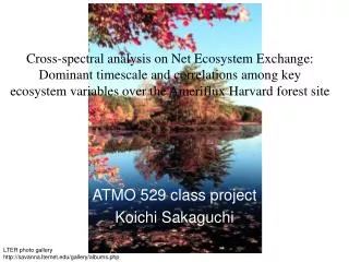
Cross-spectral analysis on Net Ecosystem Exchange: Dominant timescale and correlations among key ecosystem variables over the Ameriflux Harvard forest site. ATMO 529 class project Koichi Sakaguchi. LTER photo gallery http://savanna.lternet.edu/gallery/albums.php. Objectives.

ATMO 529 class project Koichi Sakaguchi
E N D
Presentation Transcript
Cross-spectral analysis on Net Ecosystem Exchange: Dominant timescale and correlations among key ecosystem variables over the Ameriflux Harvard forest site ATMO 529 class project Koichi Sakaguchi LTER photo gallery http://savanna.lternet.edu/gallery/albums.php
Objectives Find major frequencies (in days ~ inter-annual time scale) that explains large fraction of the variance in Net Ecosystem Exchange (CO2 flux) Find major frequencies in which NEE and another variable change together These knowledge will be helpful to infer important variables and processes that control ecosystem-level carbon cycle
Data description • Time series measured at the Harvard forest, MA • Temperate deciduous forest • Annual precipitation:756-1469 mm • Mean air temperature 6.46 °C • Eddy covariance measurement • Covariance of vertical wind and temperature or mass concentration fluctuation = vertical fluxes • Daily average values from level 4 data for 10 years period (1992 ~ 2001) Good summary by Baldocchi, 2003 in GCB
Data description • Net Ecosystem Exchange (net CO2 flux between the atmosphere and land surface) NEE = - (photosynthesis - plant respiration - soil respiration) Sign convention : downward positive http://www.atm.helsinki.fi/mikromet/
I’m having a trouble with this !!! Methods • Spectrum analysis on ecosystem CO2 flux (Net Ecosystem Exchange) time series 2. Cross-spectrum analysis on NEE and other variables: - Surface air temperature - Vapor pressure deficit - Latent heat flux - Sensible heat flux to find timescales of high correlations (Spectral Coherence) with NEE
Data preparation Gap-filling: Gaps have to be filled for harmonic analysis (Discrete Fourier transforms)(Stull, 1988)! There are about 50 days of continuous gaps in daily average data in 1992. Mean values from other 9 years are placed on this period. 2. Hanning window :Box car window is for amateurs! - decrease distortion in power spectrum from the side lobes. Fig. 6.15 in Hartmann’s note
NEE time series Mean: -0.53 gC/m2/day STD: 3.1 gC/m2/day Lag-1 autocorrelation: 0.88
Harmonic Analysis By using Fourier series in least-squares fit, we have From Hartmann’s note “Spectral Power” For a particular frequency k, Ck2 / 2 represents the fraction of the variance explained at that frequency
341 ~ 409 days 178 ~ 194 days ~90 days period Power spectrum: NEE No spectral averaging or smoothing Red line : Red noise spectrum Dashed line: statistically significant threshold with 90 & 95 % confidence
341 ~ 409 days 178 ~ 194 days ~90 days period Power spectrum: NEE Top: linear scale Bottom: semi-log plot (x-axis in log scale) No spectral averaging or smoothing Red line : Red noise spectrum Dashed line: statistically significant threshold with 90 & 95 % confidence NEE varies largely in annual & seasonal scale … not too exciting
Look at NEE anomaly Subtract 10 years mean from each daily average value. Mean: 0 gC/m2/day STD: 1.48 gC/m2/day Lag-1 autocorrelation: 0.51 Large variation concentrated in growing season
NEE anomaly power spectrum Focused on lower frequencies Top: linear scale, no smoothing Bottom: linear scale, smoothed by 5-points running mean Again most of the variance is in lower frequency. Annual ~ seasonal time scale still dominate!
NEE anomaly explained variances Significant time scale (period in days) with 95% confidence 340~510 180~220 98~105 Similar magnitudes with SSA analysis on coniferous forest in Germany (Mahecha et al., 2007) 49~51 45~45.5 1.2% 1.3% 0.8% 0.7% 0.2% % variance explained by each frequency range
Cross-spectrum analysis Analyze the power spectrum of different variables together: See how they are related in different temporal scale (covariance explained at each frequency) For two variables x(t), y(t), and their spectral power Explained covariance at a particular frequency, k is related to: “Cross spectrum” between x and y From Stull, 1988
Example: NEE & air T Intensity of in-phase signal ~ covariance ~ 90°-out-of-phase- kind-of covariance WHY? ~ Correlation Phase difference
Example: NEE & LH ~ Covariance ~ 90°-out-of-phase- kind-of covariance Tool for comparing different variables and for statistical significance ~ Correlation Phase difference
Conclusion • Processes in annual (340 ~ 400 days) and half-annual (178~194 days) time scale controls most of the variance of NEE • The variance of NEE anomaly are distributed more evenly, but still large fraction is associated with period greater than 20 days. Statistically significant periods are 340~510, 180~220, 98~105, and 49~51 days, together explains about 4% of the total variance of the anomaly. • It is demonstrated that NEE and surface air T (and LH) anomaly seem to be correlated in annual, half-annual, and 50 days periods, but statistical significance analysis needs further understanding of the speaker on cross-spectral analysis.
Future work (in one week) • Spectral coherence analysis of NEE with other variables (85%) • Temporal correlation & cross-spectral analysis of observed NEE with modeled NEE by NCAR CLM3.5 (55%) • Similar analysis on other ecosystems - arid grass-shrub land & tropical forests (40%) • Temporal correlation & cross-spectral analysis of simulated NEE with other variables from model simulation (25%) • SSA analysis on the NEE (5%) The numbers in ( ) represents the probability of finishing before the write-up due date with 95% confidence.
Supplemental material AData for cross-spectrum analysis General statistics: Row time series Anomaly
References Baldocchi, D.D, 2003. Assessing the eddy covariance technique for evaluating carbon dioxide exchange rates of ecosystems: past, present, and future. Global Change Biology,9, p479-492 Mahecha, M.D., M.Reichstein, H.Lange, N.Carvalhais, C.Bernhofer, T.Grunwald, D.Papale, and G.Seufert, 2007. Characterizing ecosystem-atmosphere interactions from short to interannual time scales. Biogeosciences, 4, p743-758. Stull, R.B. An introduction to Boundary Layer Meteorology, 1988. Kluwer Academic Press, MA, USA.