Understanding Causal Models with Directly Observed Variables
290 likes | 408 Vues
This course delves into Structural Equation Modeling (SEM) types, including Regression and Path Models, with a focus on Recursive and Nonrecursive models. Learners work through Example 7: Felson and Bohrnstedt's study on 209 girls, exploring variables like Academic, Attract, GPA, Height, Weight, and Rating. The course teaches the linear, additive, and causal assumptions of SEM. Participants learn to estimate effect parameters, decompose correlations, and assess model fit using AMOS, SPSS, and Excel. Model comparisons, Chi-square tests, AIC values, and goodness-of-fit statistics are explored to enhance understanding and application of SEM.

Understanding Causal Models with Directly Observed Variables
E N D
Presentation Transcript
SOC 681 – Causal Models with Directly Observed Variables James G. Anderson, Ph.D. Purdue University
Types of SEMs • Regression Models • Path Models • Recursive • Nonrecursive
Class Exercise: Example 7SEMs with Directly Observed Variables • Felson and Bohrnstedt’s study of 209 girls from 6th through 8th grade • Variables • Academic: Perceived academic ability • Attract: Perceived attractiveness • GPA: Grade point average • Height: Deviation of height from the mean height • Weight: Weight adjusted for height • Rating: Rating of physical attractiveness
Assumptions • Relations among variables in the model are linear, additive and causal. • Curvilinear, multiplicative and interaction relations are excluded. • Variables not included in the model but subsumed under the residuals are assumed to be not correlated with the model variables.
Assumptions • Variables are measured on an interval scale. • Variables are measured without error.
Objectives • Estimate the effect parameters (i.e., path coefficients). These parameters indicate the direct effects of a variable hypothesized as a cause of a variable taken as an effect. • Decompose the correlations between an exogenous and endogenous or two endogenous variables into direct and indirect effects. • Determine the goodness of fit of the model to the data (i.e., how well the model reproduces the observed covariances/correlations among the observed variable).
AMOS Input • ASCII • SPSS • Microsoft Excel • Microsoft Access • Microsoft FoxPro • dBase • Lotus
AMOS Output • Path diagram • Structural equations effect coefficients, standard errors, t-scores, R2 values • Goodness of fit statistics • Direct and Indirect Effects • Modification Indices.
Goodness of Fit: Model 2 • Chi-Square = 29.07 df = 15 p < 0.06 • Chi-Square/df = 1.8 • RMSEA = 0.086 • GFI = 0.94 • AGFI = 0.85 • AIC = 67.82
Chi Square: 2 • Best for models with N=75 to N=100 • For N>100, chi square is almost always significant since the magnitude is affected by the sample size • Chi square is also affected by the size of correlations in the model: the larger the correlations, the poorer the fit
Chi Square to df Ratio: 2/df • There are no consistent standards for what is considered an acceptable model • Some authors suggest a ratio of 2 to 1 • In general, a lower chi square to df ratio indicates a better fitting model
Root Mean Square Error of Approximation (RMSEA) • Value: [ (2/df-1)/(N-1) ] • If 2 < df for the model, RMSEA is set to 0 • Good models have values of < .05; values of > .10 indicate a poor fit.
GFI and AGFI (LISREL measures) • Values close to .90 reflect a good fit. • These indices are affected by sample size and can be large for poorly specified models. • These are usually not the best measures to use.
Akaike Information Criterion (AIC) • Value: 2 + k(k-1) - 2(df) where k= number of variables in the model • A better fit is indicated when AIC is smaller • Not standardized and not interpreted for a given model. • For two models estimated from the same data, the model with the smaller AIC is preferred.
Model Building • Standardized Residuals ACH – Ethnic = 3.93 • Modification Index ACH – Ethnic = 10.05
Goodness of Fit: Model 3 • Chi-Square = 16.51 df = 14 p < 0.32 • Chi-Square/df = 1.08 • RMSEA = 0.037 • GFI = 0.96 • AGFI = 0.90 • AIC = 59.87
Comparing Models • Chi-Square Difference = 12.56 df Difference = 1 p < .0005 • AIC Difference = 7.95
Difference in Chi Square Value: X2diff = X2model 1 -X2 model 2 DFdiff = DF model 1 –DFmodel 2
Class Exercise: Example 7SEMs with Directly Observed Variables • Attach the data for female subjects from the Felson and Bohrnstedt study (SPSS file Fels_fem.sav) • Fit the non-recursive model • Delete the non-significant path between Attract and Academic and refit the model • Compare the chi square values and the AIC values for the two models
Class Exercise: Example 7SEMs with Directly Observed Variables • Felson and Bohrnstedt’s study of 209 girls from 6th through 8th grade • Variables • Academic: Perceived academic ability • Attract: Perceived attractiveness • GPA: Grade point average • Height: Deviation of height from the mean height • Weight: Weight adjusted for height • Rating: Rating of physical attractiveness