Download
1 / 13
140 likes | 282 Vues
This document explores the coupling methods applied in shallow-water models for improving weather predictions. Emphasizing the Davies relaxation scheme, we analyze its effectiveness in minimizing reflection and enhancing wave characteristics through careful discretization and parameterization. The research integrates high-resolution numerical weather prediction (NWP) techniques, focusing on variable resolution models like ARPEGE and LAM. The critical evaluation of boundary conditions and relaxation zones aims to ascertain their impact on accurately simulating atmospheric processes.

E N D
Department of Meteorology & Climatology FMFI UK Bratislava Davies Couplingin a Shallow-Water Model Matúš MARTÍNI
Arakawa, A., 1984. Boundary conditions in limited-area model. Dep. of Atmospheric Sciences. University of California, Los Angeles: 28pp. • Davies, H.C., 1976. A lateral boundary formulation for multi-level prediction models. Q. J. Roy. Met. Soc., Vol. 102, 405-418. • McDonald, A., 1997. Lateral boundary conditions for operational regional forecast models; a review. Irish Meteorogical Service, Dublin: 25 pp. • Mesinger, F., Arakawa A., 1976. Numerical Methods Used in Atmospherical Models. Vol. 1, WMO/ICSU Joint Organizing Committee, GARP Publication Series No. 17, 53-54. • Phillips, N. A., 1990. Dispersion processes in large-scale weather prediction. WMO - No. 700, Sixth IMO Lecture: 1-23. • Termonia, P., 2002. The specific LAM coupling problem seen as a filter. Kransjka Gora: 25 pp.
Motivation High resolution NWP techniques: • global model with variable resolution ARPEGE 22 – 270 km • low resolution driving model with nested high resolution LAM DWD/GME DWD/LM 60 km 7 km • combination of both methods ARPEGE ALADIN/LACE ALADIN/SLOK 25 km 12 km 7 km
WHY NESTED MODELSIMPROVE WEATHER - FORECAST • the surface is more accurately characterized (orography, roughness, type of soil, vegetation, albedo …) • more realistic parametrizations might be used, eventually some of the physical processes can be fully resolved in LAM • own assimilation system better initial conditions (early phases of integration)
Shallow-water equations • 1D system (Coriolis acceleration not considered) • linearization around resting background • forward-backward scheme • centered finite differences DISCRETIZATION
Davies relaxation scheme continuous formulation inshallow-water system discrete formulation - general formalism:
PROPERTIES OF DAVIES RELAXATION SCHEME Input of the wave from the driving model u j
Difference betweennumerical and analytical solution 8-point relaxation zone (no relaxation)
Outcome of the wave, which is not represented in driving model
8-point relaxation zone analytical solution 8 72 8 72 8 8 72 8 72
Minimalization of the reflection • weight function • width of the relaxation zone • the velocity of the wave (4 different velocities satisfying CFL stability criterion) (simulation of dispersive system) • wave-length
Choosing the weight function testing criterion - critical reflection coefficient r r [%] r [%] linear convex-concave (ALADIN) cosine tan hyperbolic quartic quadratic number of points in relaxation zone
(more accurate representation of surface) DM LAM DM LAM LAM DM 8 32 8 32 8 32 DM-driving modelLAM-limited area model