Polar Low Case Study
Polar Low Case Study. Paula Doubrawa Moreira Xiangdong Zhang Jeremy Krieger Jing Zhang. Outline. What, when, where? Intro to research and methods Preliminary results Experiment 1 Experiment 2 Experiment 3 Experiment 4 Conclusion. What?. I ntense maritime mesoscale cyclones

Polar Low Case Study
E N D
Presentation Transcript
Polar Low Case Study Paula DoubrawaMoreira Xiangdong Zhang Jeremy Krieger Jing Zhang
Outline • What, when, where? • Intro to research and methods • Preliminary results • Experiment 1 • Experiment 2 • Experiment 3 • Experiment 4 • Conclusion
What? • Intensemaritimemesoscalecyclones • Formpolewardof a major barocliniczone • Mostlydue to strongcoldinflowsofdry/stableArcticair over warmerwatersurfaces • Scalesup to 1000km (621mi) • Near-surfacewindsexceeding 15m/s (33mph) Definitions by: - Kolstad, E. W. (2007), Extreme winds in the Nordic Seas: polar lows and Arctic fronts in a changing climate, University of Bergen, Bergen. - European Geophysical Society’s Polar Low Working Group, Rasmussen, E. A. T., J. (2003), Polar Lows: Mesoscale Weather Systems in the Polar Regions, 624 pp., Cambridge University Press, Cambridge, Cambridge.
When? October 9th 2009 Formed in themorning ~ 1100 AKDT Reachedmaturity in afternoon ~ 1600 AKDT Starteddissipatingatnight ~ 2100 AKDT • Scale of the system ≈ 9° lat x 20° lon ≈ 1000km x 800km = 621mi x 501mi Oct 10th 2009 01:33 UTC (Oct 9th 1700 AKDT) Oct 9th 2009, 1633 UTC (0800 AKDT) Satelliteimageon IR channelfromthe DMS (DefenseMeteorologicalSatelliteProgram) OLS (OperationalLinescan System) sensor.
Where? • ChukchiSea, western Beaufort Sea • Centered to the NW ofBarrow, AK • Regionwithconsiderableminimumofcylclonefrequencyandintensitywhencompared to otherregionsoftheArctic[Lynch, 2003] • Only published record of a polar-like disturbance in this region is by Twitchell [1989] about a system in October 1985 Lynch, A. H., E. N. Cassano, J. J. Cassano, and L. R. Lestak (2003), Case Studies of High Wind Events in Barrow, Alaska: Climatological Context and Development Processes, Monthly Weather Review, 131(4), 719-732. Twitchell, P. F. (1989), Polar and Arctic lows / edited by Paul F. Twitchell, Erik A. Rasmussen, and Kenneth L. Davidson, A. Deepak Pub, Hampton, Va., USA :.
Research goals • Use modelingtechniques to understandphysicallyanddynamicallywhatledto developmentofthis polar low • Determine themostsuitablemodel setup for forecastingthiskindof system in thisarea
Some model configurations • Weather Research and Forecasting model [Michalakes et al., 2001] • 2-way nesting : 2 domains with different resolutions are run simultaneously and communicatively • Resolutions 18km, 6km • Interpolation to 40 vertical levels • Initialization October 8th 2009 at 1200UTC • Run for60h Michalakes, J., S. Chen, J. Dudhia, L. Hart, J. Klemp, J. Middlecoff, and W. Skamarock (2001): Development of a Next Generation Regional Weather Research and Forecast Model. Developments in Teracomputing: Proceedings of the Ninth ECMWF Workshop on the Use of High Performance Computing in Meteorology. Eds. Walter Zwieflhofer and Norbert Kreitz. World Scientific, Singapore. pp. 269-276.
Past/Present Research • Accomplished : modeling experiments Purpose: obtain solid simulation for further analysis assess model sensitivies/forecasting capabilities • Current work : Statistical evaluation of the obtained simulations • Experiment 1: Sensitivity to initialconditions: 4 simulationsusingdifferentreanalysisdatasets • Experiment 2: Sensitivity to physicalparameterizations: 10 ensemble membersandan ensemble meanvaryingmicrophysics, radiation, surfacelayer, boyndarylayerandconvectionschemes • Experiment 3: Sensitivity to initialization time: 5 simulations starting atdifferent times
Data for model verification • Network of surface data being used for model verification
Statistical parameters for model verification • Bias = • RMSE = • URMSE = Systematic errors resulting from model parameters, deficiencies, approximations Evaluates overall performance; sensitive to systematic and large errors Like the former but getting rid of the bias.
Experiment 1: Sensitivity to IC • Same simulation setup • 4 different reanalysis datasets as input for initial and boundary conditions • NCEP Reanalysis 1 (NNRP1) • NCEP Reanalysis 2 (NNRP2) • European Interim Reanalysis (ERA) • Japanese Reanalysis (JRA)
Just to give a broad “spatial” view of error magnitudes… Speed: from x<2 m/s to x>15 m/s Direction: from x<45° to x>315
Domain-averaged statistics • RMSE and URMSE averaged over all times and all 205 stations • Loss of spatial variability evens out errors among different simulations
Domain-averaged statistics • Bias for each simulation time averaged over all 205 stations • Same problem can be seen spatial averages are not ideal for evaluating differences among the simulations.
Solution : look separately at each station • Selected sub-domain • Will show data for 5 stations very close to storm area Shell Beaufort Buoy Milne Point Barrow Deadhorse Reindeer Island
Obs/Modeled+ σ surface wind speeds • 4 simulations, 1 point • Shell Beaufort Buoy (70.372N, 146.062W) • ERA captures reality better
Obs/Modeled + σ surface wind speeds • 4 points, 1 simulation • ERA Simulation
Errors for same 4 points and 4 simulations ERA : smaller RMSE for all 5 points
Experiment 2: Sensitivity to physical parameterizations • Only ERA as IC • 10 different combination of physics • Not yet evaluated using station data • Preliminary assessment using reanalysis product indicates that • Ensemble Member 1 presents significantly smaller errors and biasesfor various atmospheric parameters • (wind speed and direction, sea-level pressure, relative humidity, geopotentialheight, air temperature)
Experiment 3: Sensitivity to initialization time • Used setup of Ensemble Member 1 from previous Experiment • 5 starting times, 6 hours apart • Preliminary assessment indicates solid simulation – errors do not vary with initialization time Ensemble Member 1 from Experiment 2 ERA simulation from Experiment 1 5 simulations starting at different times Average of these 5 Temp. at 500hPa SLP RH at 850hPa
Experiment 3: Sensitivity to initialization time • Model output for the best-performing simulation • Temperature at 2m • Wind at 10m • SLP Strong E, SE winds Beaufort High Polar Low Aleutian Low
Experiment 4: Sensitivity to initialization time • Same as Experiment 3 but for model setup of ERA Simulation from Experiment 1 • Preliminary assessment shows that simulation was sensitive to initialization time – not stable (unlike Experiment 3) Temp. at 500hPa SLP RH at 850hPa
Conclusions • According to preliminary analysis: • ERA seems to be the best performing reanalysis dataset for WRF input • A solid simulation can be achieved using ERA-Interim IC/BC and specific physical parameterizations combinations (that used for member 1 of Experiment 2)
Thank you. pmoreira@alaska.edu

